第 48 章 随机截距模型中加入共变量
这一章我们来把随机截距模型加以扩展,在固定效应部分增加想要调整的共变量。
48.1 多元线性回归模型的延伸
如果有一个含有两个预测变量的多元线性回归模型:
\[ \begin{equation} Y_{ij} = \beta_0 + \beta_1 X_{1ij} + \beta_2 X_{2ij} + \epsilon_{ij} \end{equation} \tag{48.1} \]
如果观测数据内部具有嵌套式结构,也就是有些对象之间有相关性,有些对象之间没有,那么上面这个多元线性回归模型的误差项\(\epsilon_{ij}\) 其实是不能被认为相互独立的,因为数据中处以同一层的个体之间互相有关联性(属于同一所学校的学生之间,同一所医院的病人之间)。但是于此同时,我们不妨把最后的误差项分成两个部分
\[ \epsilon_{ij} = u_j + e_{ij} \]
其中,
- \(u_j\),是在随机截距模型中用到的随机截距部分,\(u_j \sim N(0, \sigma_u^2)\),它允许不同层的数据有自己的截距;
- \(e_{ij}\),是剥离掉层内相关 (等同于层间相异,intra-class correlation = between-class heterogeneity) 之后,剩余的随机残差;
之后把式子 (48.1) 重新整理,就遇到了我们似曾相识的随机截距模型:
\[ \begin{equation} Y_{ij} = (\beta_0 + u_j) + \beta_1 X_{1ij} + \beta_2 X_{2ij} + e_{ij} \end{equation} \tag{48.2} \]
这就是一个混合效应线性回归模型 (linear mixed model)。其中,
- 固定效应部分的参数有 fixed effect parameters: \(\beta_0, \beta_1, \beta_2\);
- 随机效应部分的参数有 random effect parameters: \(u_j, e_{ij}\)。
但是和之前的随机截距模型不同的是,这里我们在固定效应部分增加了两个共变量\(X_1, X_2\),所以从该模型作出的所有统计推断,都是建立在以这两个共变量为条件的基础之上的(conditionally on \(\mathbf{X} = \{ X_1, X_2\}\))。所以对于 \(u_j, e_{ij}\),他们的前提条件就变成了:
- \(\text{E}(u_j|\mathbf{X} = \{ X_1, X_2\}) = 0\);
- \(\text{E}(e_{ij}|\mathbf{X} = \{ X_1, X_2, u_j\}) = 0\)。
根据这两个条件,我们可以继续得到:
- \(\text{E}(e_{ij} | \mathbf{X} = \{ X_1, X_2\}) = 0\);
- \(\text{E}(Y_{ij} | \mathbf{X} = \{ X_1, X_2\}) = \beta_0 + \beta_1X_{1ij} + \beta_2X_{2ij}\)
也就是说,这个包含了 \(u_j, e_{ij}\) 的多元线性回归模型,其边际模型 (marginal regression over \(u_j, e_{ij}\)) 还是一个线性回归。
注意
- 模型的固定效应部分加入了多个共变量\(\mathbf{X} = \{ X_1, X_2\}\) 之后,模型所估计的层内相关系数(intra-class correlation, \(\lambda\)) 也成了以这些共变量为条件的层内相关系数。
- \(u_j\) 这个层别随机截距 (cluster-specific random intercept) 此时会囊括已知/未知的层水平的特征 (class-level characteristics, i.e. unmeasured heterogeneity between clusters)。它会随着你在模型中加入层水平的解释变量而逐渐变小 (Its size will decrease as more explanatory variables for the cluster difference are included in the model)。
48.2 siblings 数据中新生儿体重的实例
在数据 silblings 中,研究者收集了来自 3978 名母亲,8604 名新生儿出生体重 (g) 的数据。此外,该数据中还收集了这些新生儿的胎龄 (week),新生儿的性别,母亲孕期的吸烟状况,以及怀孕时母亲的年龄。在这个数据里,每个母亲是该数据的第二阶层 (level 2),每个母亲的相关信息,就是属于第二阶层的层水平数据。每个新生儿的体重和相关数据,就是第一阶层 (level 1) 数据,一个母亲可能生 1-3 个婴儿,这些来自同一个母亲的新生儿之间很显然不能视之为相互独立。研究者关心一个固定效应部分不包含其他共变量的随机截距模型(the Null Model),和固定效应部分增加了其他共变量的随机截距模型(the Full Model) 哪个更能解释这个数据或者更好的拟合这个数据(better fitting the data)。
下面就先把数据读入 R,然后建立一个零模型 (the Null Model):
library(haven)
library(tidyverse)
library(nlme)

siblings <- read_dta("../Datas/siblings.dta")
M0 <- lme(fixed = birwt ~ 1, random  = ~ 1 | momid, data = siblings, method = "REML")
summary(M0)
## Linear mixed-effects model fit by REML
## Data: siblings
## AIC BIC logLik
## 130951.2 130972.4 -65472.6
##
## Random effects:
## Formula: ~1 | momid
## (Intercept) Residual
## StdDev: 368.356 377.6577
##
## Fixed effects: birwt ~ 1
## Value Std.Error DF t-value p-value
## (Intercept) 3467.969 7.138555 4626 485.8082 0
##
## Standardized Within-Group Residuals:
## Min Q1 Med Q3 Max
## -6.274306389 -0.486019398 0.003529979 0.505355037 4.050392366
##
## Number of Observations: 8604
## Number of Groups: 3978## Model df AIC BIC logLik Test L.Ratio p-value
## M0 1 3 130951.2 130972.4 -65472.60
## M0_fixed 2 2 132265.3 132279.4 -66130.66 1 vs 2 1316.117 <.0001下一步,我们来对该数据拟合一个全模型(the Full Model),我们可以先对两个连续型变量(胎龄,gestational age 和母亲怀孕时年龄,maternal age) 进行适当的转换,比方说把胎龄标准化成38 周,怀孕时年龄标准化成30 岁:
siblings <- siblings %>%
  mutate(c_gestat = gestat - 38, # centering gestational age to 38 weeks
         c_mage = mage - 30,  # centering maternal age to 30 years old
         male = factor(male, labels = c("female", "male")),
         smoke = factor(smoke, labels = c("Nonsmoker", "Smoker")))
#M_full <- lme(fixed = birwt ~ c_gestat + male + smoke + c_mage, random  = ~ 1 | momid, data = siblings, method = "REML")
M_full <- lme4::lmer(birwt ~ c_gestat + male + smoke + c_mage + (1 | momid), data = siblings, REML = TRUE)
library(lmerTest)
summary(M_full)
## Linear mixed model fit by REML ['lmerMod']
## Formula: birwt ~ c_gestat + male + smoke + c_mage + (1 | momid)
## Data: siblings
##
## REML criterion at convergence: 128984.9
##
## Scaled residuals:
## Min 1Q Median 3Q Max
## -4.1459 -0.5288 -0.0087 0.5359 3.6329
##
## Random effects:
## Groups Name Variance Std.Dev.
## momid (Intercept) 99784 315.9
## Residual 118012 343.5
## Number of obs: 8604, groups: momid, 3978
##
## Fixed effects:
## Estimate Std. Error t value
## (Intercept) 3341.096 8.664 385.62
## c_gestat 85.424 2.161 39.53
## malemale 133.948 8.869 15.10
## smokeSmoker -239.999 15.979 -15.02
## c_mage 13.158 1.090 12.07
##
## Correlation of Fixed Effects:
## (Intr) c_gstt maleml smkSmk
## c_gestat -0.347
## malemale -0.535 0.038
## smokeSmoker -0.244 0.017 0.006
## c_mage 0.137 0.020 -0.001 0.145从全模型的结果报告中可以看出,固定效应部分加入的所有解释变量都是有意义的。他们的含义如下:
c_gestat 85.42: 当模型中的其他变量保持不变时(当模型中其他的变量被调整时),胎龄每增加一周,无论是同一个妈妈还是不同妈妈(either from the same or another mother, i.e. in any cluster) 生下的新生儿的出生体重增加的期待值是85.42 g。male 133.95: 新生儿的性别如果是男孩,无论是同一个妈妈还是不同妈妈生下的新生儿,他的出生体重会比女孩增加 133.95 g。
再看这两个模型的随机效应部分,无论是第二层级水平的层标准差(cluster-level) 还是第一层级(elementary-level) 的标准差都随着固定效应部分加入新的解释变量而变小。我们同样可以用极大似然法 (ML) 拟合这两个模型,其方差大小总结成下面的表格:
| Random Effect | Null Model | Full Model | Null Model | Full Model |
|---|---|---|---|---|
| u | 368.3558 | 315.8853 | 368.2864 | 315.7320 |
| e | 377.6577 | 343.5296 | 366.6579 | 343.4581 |
表格的右半部分总结的是使用极大似然法 (会偏小估计随机效应方差),其实它们和 REML 法估计的结果相差不大。 值得强调的是,由于REML 法每次估计的数据是去除掉固定效应部分以后的随机误差部分的数据,所以当两个用REML 法估计的混合效应模型其固定效应部分不一致的时候,这两个模型实际拟合了不同的数据,是不能使用LRT 来比较两个模型哪个更好的。
48.3 赋值予随机效应成分
值得建议地,拟合了任何一个混合效应模型以后,需要尽量避免直接跳入结论陈述阶段,而应当先对模型是否符合其假定的前提条件进行模型诊断。而且,对模型的拟合后截距及其层级随机效应 (cluster random effect) 进行视觉化展现变得十分有用。
总体来说,有两种方法可以用于估计并提取这些拟合值 – ML 和 Empirical Bayes (EB)。
48.3.1 简单预测 simple prediction
和简单线性回归模型一样,我们可以计_算模型的预测值和观测值之间的差,获得一个包含了两个随机效应成分的量:
\[ \begin{aligned} Y_{ij} & = \beta_0 + \beta_1X_{1ij} + u_j + e_{ij} \\ \Rightarrow Y_{ij} & = \beta_0 + \beta_1X_{1ij} + \epsilon_{ij} \\ \Rightarrow \hat\epsilon_{ij} & = Y_{ij} - (\hat\beta_0 + \beta_1X_{1ij}) \end{aligned} \]
那么最简单的方法就是计算了这个随机效应成分的混合体之后,对其取平均值,作为 \(u_j\) 的简单估计:
M_full <- lme(fixed = birwt ~ c_gestat + male + smoke + c_mage, random  = ~ 1 | momid,
              data = siblings, method = "REML")

siblings$yhat <- M_full$fitted[,1]
siblings <- siblings %>%
  mutate(res = birwt- yhat)
Mean_siblings <- plyr::ddply(siblings, ~momid, summarise, uhat = mean(res))
Mean_siblings[Mean_siblings$momid == 14,]
## momid uhat
## 1 14 105.124## # A tibble: 3 × 5
## momid gestat birwt yhat res
## <dbl> <dbl> <dbl> <dbl> <dbl>
## 1 14 24 2790 1961. 829.
## 2 14 42 2693 3512. -819.
## 3 14 39 3600 3295. 305.找到编号 14 号的母亲,她有三个孩子被研究者记录到,他们中有的孩子使用该模型计算的拟合值 (fitted value = yhat) 并不准确。在调整了胎龄,婴儿性别,母亲的吸烟状况,和母亲怀孕时年龄后,该母亲生的孩子,和该队列的总体平均值 (overall mean) 相比较,其偏差达到了 105.12 g。
我们可以对每个母亲的拟合偏差做总结归纳:
Mean_siblings %>%
  summarise(Mean_uhat = mean(uhat),
            sd_uhat = sd(uhat),
            min_uhat = min(uhat),
            max_uhat = max(uhat))
## Mean_uhat sd_uhat min_uhat max_uhat
## 1 -0.5115952 395.0677 -1386.937 1772.721可见这 3978 名母亲总体的拟合偏差的均值为 -0.511,接近零。且它的标准差接近 400。这样一种直接利用观测值和拟合值之差做曾内平均的方法被叫做极大似然法 ML,这样计算获得的平均偏差被标记为 \(\hat u_j^{\text{ML}}\)
48.3.2 EB 预测值
EB 法 (经验贝叶斯法) 也一样要利用拟合模型后的 \(\beta\) 来计算获得层残差 (cluster level residuals)。但是用 EB 法时我们还再使用层残差的一个前提条件: \(u_j \sim N(0, \sigma_u^2)\)。在线性随机截距模型中,EB 法计算的层级残差和简单法计算的层残差之间有如下的简单转换关系:
\[ \hat u_j^{\text{EB}} = \hat R_j\hat u_j^{\text{ML}} \]
其中\(\hat R_j\) 被定义为ML 法计算层级残差的可靠性(reliability of \(\hat u_j^{\text{ML}}\)),它是一个包含了层级方差和个人水平方差的方程:
\[ \hat R_j = \frac{\hat\sigma_u^2}{\hat\sigma_u^2 + \sigma_e^2/n_j} = \hat w_j \hat \sigma_u^2 \]
其中 \(\hat w_j\) 是之前在章节 47.4.1 定义的权重。这个\(\hat R_j\) 又被叫做是收缩因子(shrinkage factor),因为它取值是在0 到1 之间,所以它会把ML 法计算获得的层级误差按照收缩银子比例收缩变小。当 \(\sigma_u\) 本身比较小,或者个体的随机误差大 \(\sigma_e\),或者层内样本量小 \(n_j\) 时收缩因子的作用更大。
此时,预测误差 \((\hat u_j^{\text{EB}} - u_j)\) 才是我们能够从观测数据以及模型中获得的均值为零方差又最小的残差。所以 \(\hat u_j^{\text{EB}}\) 又被称为 \(\text{Best linear unbiased predictors, BLUP}\)。
第二层级残差的方差是:
\[ R_j\hat \sigma_u^2 \]
48.4 混合效应模型的诊断
辛苦计算了 BLUP 之后,就可以拿它,和模型的标准化残差来对模型作出一定的诊断。由于计算获得的 BLUP 方差不齐,要先对其标准化之后再作正态图:
# the standardized

n_child <- siblings %>% count(momid, sort = TRUE)
Mean_siblings <- merge(Mean_siblings, n_child, by = "momid")

Mean_siblings <- Mean_siblings %>%
  mutate(# extract the random effect (EB) residuals at level 2
         uhat_eb = ranef(M_full)$`(Intercept)`,
         # shrinkage factor
         R = 315.7338^2/(315.7338^2 + (343.4572^2)/n),
         # Empirical Bayes prediction of variance of uhat
         var_eb = R*(315.7338^2),
         # standardize the EB uhat
         uhat_st = uhat_eb/sqrt(var_eb)
  )

# 计算每个个体的标准化残差

siblings$ehat <- residuals(M_full, level = 1, type = "normalized")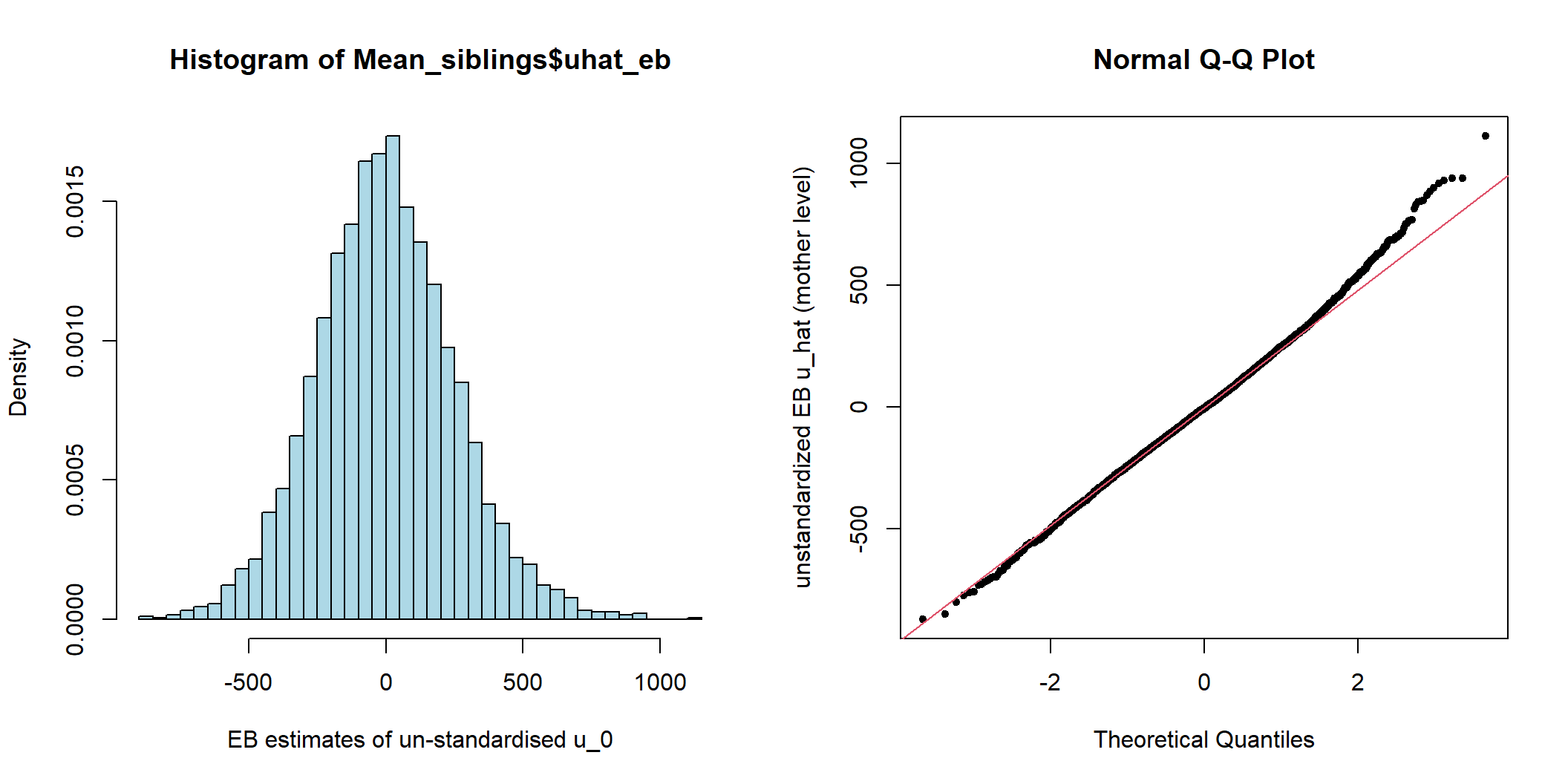
图 48.1: Histogram and Q-Q plot of cluster (mother) level unstandardized residuals for the intercept

图 48.2: Histogram and Q-Q plot of cluster (mother) level standardized residuals for the intercept
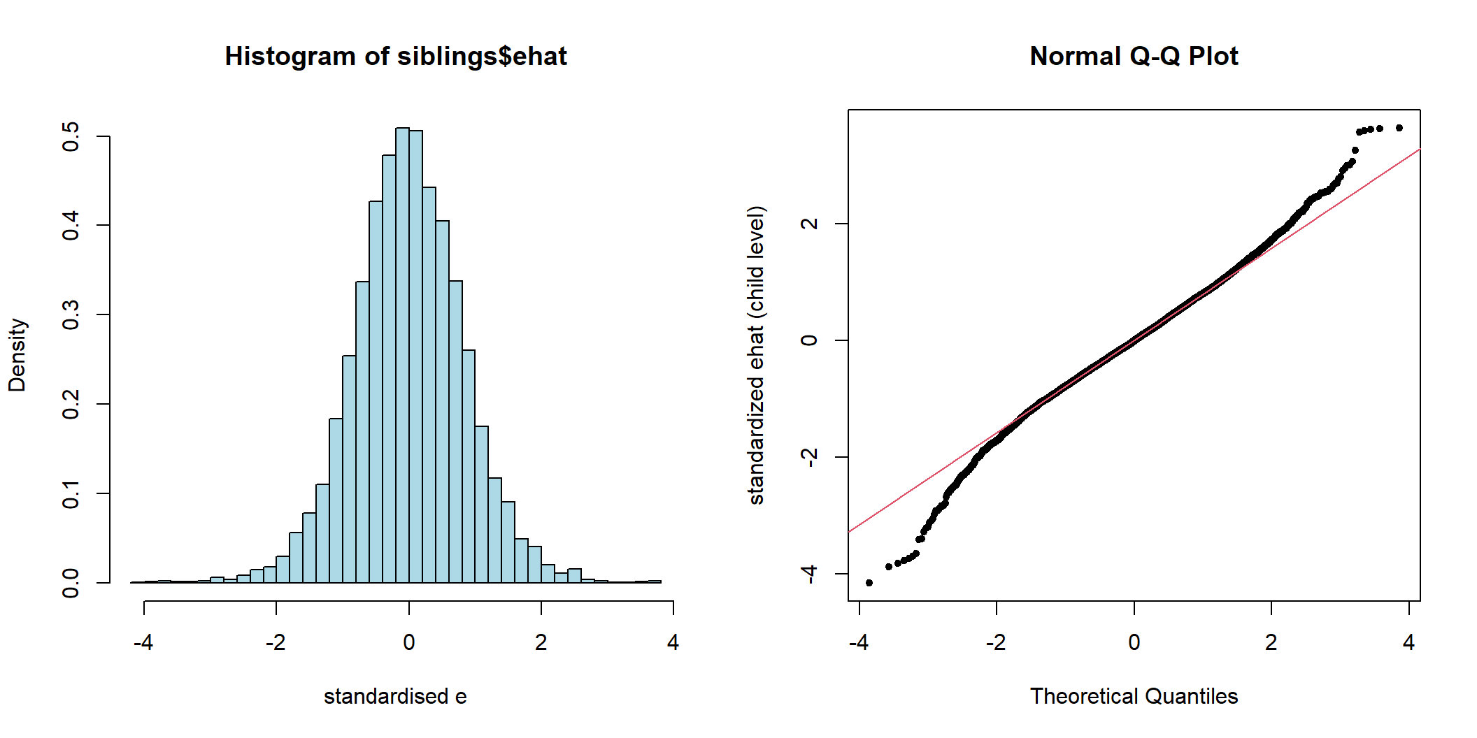
图 48.3: Histogram and Q-Q plot of individual (pupil) level standardized residuals for the intercept
这些正态图,主要用于辅助寻找看哪里有异常值 (outliers)。
48.5 第二层级 (cluster level/level 2) 的协方差
还是这个siblings 数据中,关于母亲的数据在该母亲生的孩子中是保持不变的,比如有人种(black),母亲受教育情况(hsgrad),和母亲的婚姻状况( married)。因为这些变量属于解释第二层级 (level 2) 的变量,加入这些变量在固定效应部分只能解释层间的方差 (between clusters variance):
siblings <- siblings %>%
  mutate(black = factor(black, labels = c("No", "Yes")),
         hsgrad = factor(hsgrad, labels = c("No", "Yes")),
         married = factor(married, labels = c("No", "yes")))

M_full1 <- lmer(birwt ~ c_gestat + male + smoke + c_mage + black + married + hsgrad + (1 | momid),
                data = siblings, REML = TRUE)
summary(M_full1)
## Linear mixed model fit by REML. t-tests use Satterthwaite's method [
## lmerModLmerTest]
## Formula: birwt ~ c_gestat + male + smoke + c_mage + black + married +
## hsgrad + (1 | momid)
## Data: siblings
##
## REML criterion at convergence: 128884.7
##
## Scaled residuals:
## Min 1Q Median 3Q Max
## -4.1931 -0.5322 -0.0124 0.5412 3.6530
##
## Random effects:
## Groups Name Variance Std.Dev.
## momid (Intercept) 96846 311.2
## Residual 118053 343.6
## Number of obs: 8604, groups: momid, 3978
##
## Fixed effects:
## Estimate Std. Error df t value Pr(>|t|)
## (Intercept) 3297.461 23.304 4601.176 141.500 < 2e-16 ***
## c_gestat 84.456 2.158 7887.403 39.128 < 2e-16 ***
## malemale 133.789 8.851 7160.407 15.115 < 2e-16 ***
## smokeSmoker -227.942 16.332 7674.001 -13.956 < 2e-16 ***
## c_mage 11.038 1.141 5488.409 9.672 < 2e-16 ***
## blackYes -177.895 25.971 3912.412 -6.850 8.55e-12 ***
## marriedyes 61.172 22.279 4164.232 2.746 0.00606 **
## hsgradYes -4.212 13.979 3949.604 -0.301 0.76321
## ---
## Signif. codes: 0 '***' 0.001 '**' 0.01 '*' 0.05 '.' 0.1 ' ' 1
##
## Correlation of Fixed Effects:
## (Intr) c_gstt maleml smkSmk c_mage blckYs mrrdys
## c_gestat -0.111
## malemale -0.204 0.038
## smokeSmoker -0.287 0.009 0.008
## c_mage 0.222 0.034 -0.004 0.071
## blackYes -0.377 0.041 0.007 0.064 0.036
## marriedyes -0.914 -0.025 0.007 0.227 -0.230 0.348
## hsgradYes -0.165 0.011 -0.012 -0.044 0.172 -0.046 0.016加入了第二层级协变量之后, \(\sigma^2_u = 96845.79\),相比没加之前的小了一些 \((\sigma^2_{u} = 99784)\)。但是 \(\sigma^2_e\) 几乎保持不变。
48.6 层内层间效应估计
如有某个想加入模型的变量是属于第一层级的,例如 siblings 数据中的胎龄,即使是同一个妈妈生的婴儿,其出生时的胎龄也是各不相同。但是这样在模型输出的报告中,胎龄这一变量的估计量其实是其他变量保持不变时,**每增加一周胎儿对不论是同一个母亲还是不同母亲生的婴儿的出生体重的影响* *,怎样才能把同一母亲不同胎龄的影响(within effect) 和不同母亲不同胎龄的影响(between effect) 给区分出来呢?
其实很简单,我们来把胎龄这个变量做个分解:
\[ Y_{ij} = \beta_0 + \beta_{1B} \bar{X}_{\cdot j} + \beta_{1W} (X_{ij} - \bar{X}_{\cdot j}) + u_j + e_{ij} \]
把胎龄这个变量分解成\(\bar{X}_{\cdot j}\) (每个母亲生的婴儿的平均胎龄),和\(X_{ij} - \bar{X}_{\cdot j }\) (每个母亲内,每个胎儿的胎龄和平均胎龄之差) 两个部分,就解决了区分层间效应\((\beta_{1B})\) 和层内效应\((\beta_{1W })\)。的方法。下面的模型在固定效应部分只使用了胎龄一个变量 (为了这里输出报告简洁明了):
M_gestat <- lme4::lmer(birwt ~ c_gestat + (1 | momid), data = siblings, REML = TRUE)
summary(M_gestat)
## Linear mixed model fit by REML ['lmerMod']
## Formula: birwt ~ c_gestat + (1 | momid)
## Data: siblings
##
## REML criterion at convergence: 129638.4
##
## Scaled residuals:
## Min 1Q Median 3Q Max
## -3.9566 -0.5295 0.0066 0.5264 3.9872
##
## Random effects:
## Groups Name Variance Std.Dev.
## momid (Intercept) 113073 336.3
## Residual 124282 352.5
## Number of obs: 8604, groups: momid, 3978
##
## Fixed effects:
## Estimate Std. Error t value
## (Intercept) 3358.544 7.184 467.50
## c_gestat 83.732 2.231 37.52
##
## Correlation of Fixed Effects:
## (Intr)
## c_gestat -0.406当把胎龄作为一个变量放进模型的固定效应部分时,不论是不是同一个母亲生下的胎儿,只要胎龄每增加一周,出生体重就增加 83.7 g。下一个模型中,我们来把胎龄这个变量分解成层间变量和层内变量:
Mean_gestat <- plyr::ddply(siblings, ~ momid, summarise, mean_gestat = mean(gestat))
# 把每个母亲的胎儿胎龄均值 (level 2 mean) 赋予原有的数据中
avegest <- NULL
for (i in 1:3978){
  avegest <- c(avegest, rep(Mean_gestat$mean_gestat[i], with(siblings, table(momid))[i]))
}
siblings$avegest <- avegest
rm(avegest)
# 计算层内胎儿胎龄与其层均值的差异
siblings <- siblings %>%
  mutate(c_avegest = avegest - 38,
         difgest = gestat - avegest)

siblings[siblings$momid == 14,c(1,2,5,6,18:20)]
## # A tibble: 3 × 7
## momid idx gestat birwt avegest c_avegest difgest
## <dbl> <dbl> <dbl> <dbl> <dbl> <dbl> <dbl>
## 1 14 1 24 2790 35 -3 -11
## 2 14 2 42 2693 35 -3 7
## 3 14 3 39 3600 35 -3 4# 下面用 c_avegest 和 difgest 代替 gestat 放入同样模型的固定效应部分
M_gestat_sep <- lme4::lmer(birwt ~ c_avegest + difgest + (1 | momid), data = siblings, REML = TRUE)
summary(M_gestat_sep)## Linear mixed model fit by REML ['lmerMod']
## Formula: birwt ~ c_avegest + difgest + (1 | momid)
## Data: siblings
##
## REML criterion at convergence: 129557.3
##
## Scaled residuals:
## Min 1Q Median 3Q Max
## -4.0218 -0.5245 0.0094 0.5232 3.9895
##
## Random effects:
## Groups Name Variance Std.Dev.
## momid (Intercept) 111117 333.3
## Residual 123670 351.7
## Number of obs: 8604, groups: momid, 3978
##
## Fixed effects:
## Estimate Std. Error t value
## (Intercept) 3320.008 8.383 396.03
## c_avegest 113.218 4.029 28.10
## difgest 70.935 2.665 26.61
##
## Correlation of Fixed Effects:
## (Intr) c_vgst
## c_avegest -0.628
## difgest 0.000 0.000把胎龄分解了以后,从模型的输出结果可以看出,层间效应 113 g (不同的母亲),要大于层内效应 70.9 g (同一母亲不同胎儿)。
比较分解胎龄以后的模型 M_gestat_sep 和把胎龄作为一个变量的模型 M_gestat 哪个更优,可以有两种检验法:
## Data: siblings
## Models:
## M_gestat: birwt ~ c_gestat + (1 | momid)
## M_gestat_sep: birwt ~ c_avegest + difgest + (1 | momid)
##              npar    AIC    BIC logLik deviance  Chisq Df Pr(>Chisq)
## M_gestat        4 129655 129684 -64824   129647
## M_gestat_sep    5 129581 129617 -64786   129571 76.219  1  < 2.2e-16 ***
## ---
## Signif. codes: 0 '***' 0.001 '**' 0.01 '*' 0.05 '.' 0.1 ' ' 1## Linear hypothesis test
##
## Hypothesis:
## c_avegest - difgest = 0
##
## Model 1: restricted model
## Model 2: birwt ~ c_avegest + difgest + (1 | momid)
##
## Df Chisq Pr(>Chisq)
## 1
## 2 1 76.6 < 2.2e-16 ***
## ---
## Signif. codes: 0 '***' 0.001 '**' 0.01 '*' 0.05 '.' 0.1 ' ' 1无论是哪种检验,都告诉我们把胎龄分解了的模型更好。了解更多层内层间回归模型,参照 (Mann, De Stavola, and Leon 2004)。
48.7 到底选择固定还是混合模型?
目前为止我们讨论了嵌套式数据可以使用固定效应模型分析,也可以使用混合效应模型来拟合,那么到底你该选择哪个来解释你的数据呢?选择模型永远是一个很难回答的问题。哪种模型更加恰当 (appropriate) 其实要取决于你的数据结构,分层的数据的话层的数量是不是足够多?以及最重要的,你的**分析目的*。
- 如果模型中想分析的层/群组,可以被视为唯一的实体(uniqe entity,例如不同的种族),而且我们希望从模型来获得对不同种群或者不同个体中每一个个体的估计,那么固定效应模型是合适的。
- 如果层/群组其实是人群中的样本(samples from a real population,如例题中的母亲层级,人群众可以有许许多多的母亲),我们打算从这个模型的结果去推论整个人群,那么随机效应模型才是最合适的。
- 如果说层级本身的样本量(n of clusters) 太小,那么强行使用混合效应模型的话会导致随机效应的估计结果十分地低效,甚至没有意义; 当然如果你的混合效应模型关心的是固定效应部分,那么增加一些层级随机效应应该也能达到提升统计估计效率的目的。
- 如果我们关心的是层级协变量的效应,那么随机效应模型是唯一的选择。
48.8 Hierarchical例3
48.8.1 High-school-and-Beyond 数据
hsb_selected <- read_dta("../Datas/hsb_selected.dta")
length(unique(hsb_selected$schoolid)) ## number of school = 160
## [1] 160## create a subset data with only the first observation of each school
hsb <- hsb_selected[!duplicated(hsb_selected$schoolid), ]
## about 44 % of the schools are Catholic schools
with(hsb, tab1(sector, graph = FALSE, decimal = 2))## sector :
## Frequency Percent Cum. percent
## 0 90 56.25 56.25
## 1 70 43.75 100.00
## Total 160 100.00 100.00## among all the schools, average school size is 1098
hsb %>%
summarise(N = n(),
Mean = mean(size),
sd_size = sd(size),
min_size = min(size),
max_size = max(size))## # A tibble: 1 × 5
## N Mean sd_size min_size max_size
## <int> <dbl> <dbl> <dbl> <dbl>
## 1 160 1098. 630. 100 2713## among all the pupils, about 53% are females
with(hsb_selected, tab1(female, graph = FALSE, decimal = 2))## female :
## Frequency Percent Cum. percent
## 0 3390 47.18 47.18
## 1 3795 52.82 100.00
## Total 7185 100.00 100.00## among all the pupils, about 27.5% are from ethnic minorities
with(hsb_selected, tab1(minority, graph = FALSE, decimal = 2))## minority :
## Frequency Percent Cum. percent
## 0 5211 72.53 72.53
## 1 1974 27.47 100.00
## Total 7185 100.00 100.0048.8.2 拟合两个随机截距模型 (ML, REML),结果变量用 mathach,解释变量用 ses。观察结果是否不同。
library(lme4)
Fixed_reml <- lmer(mathach ~ ses + (1 | schoolid), data = hsb_selected, REML = TRUE)
summary(Fixed_reml)
## Linear mixed model fit by REML. t-tests use Satterthwaite's method [
## lmerModLmerTest]
## Formula: mathach ~ ses + (1 | schoolid)
## Data: hsb_selected
##
## REML criterion at convergence: 46645.2
##
## Scaled residuals:
## Min 1Q Median 3Q Max
## -3.12607 -0.72720 0.02188 0.75772 2.91912
##
## Random effects:
## Groups Name Variance Std.Dev.
## schoolid (Intercept) 4.768 2.184
## Residual 37.034 6.086
## Number of obs: 7185, groups: schoolid, 160
##
## Fixed effects:
## Estimate Std. Error df t value Pr(>|t|)
## (Intercept) 12.6575 0.1880 148.3022 67.33 <2e-16 ***
## ses 2.3902 0.1057 6838.0776 22.61 <2e-16 ***
## ---
## Signif. codes: 0 '***' 0.001 '**' 0.01 '*' 0.05 '.' 0.1 ' ' 1
##
## Correlation of Fixed Effects:
## (Intr)
## ses 0.003Fixed_ml <- lmer(mathach ~ ses + (1 | schoolid), data = hsb_selected, REML = FALSE)
summary(Fixed_ml)## Linear mixed model fit by maximum likelihood . t-tests use Satterthwaite's
## method [lmerModLmerTest]
## Formula: mathach ~ ses + (1 | schoolid)
## Data: hsb_selected
##
## AIC BIC logLik deviance df.resid
## 46649.0 46676.5 -23320.5 46641.0 7181
##
## Scaled residuals:
## Min 1Q Median 3Q Max
## -3.1263 -0.7277 0.0220 0.7578 2.9186
##
## Random effects:
## Groups Name Variance Std.Dev.
## schoolid (Intercept) 4.729 2.175
## Residual 37.030 6.085
## Number of obs: 7185, groups: schoolid, 160
##
## Fixed effects:
## Estimate Std. Error df t value Pr(>|t|)
## (Intercept) 12.6576 0.1873 149.1760 67.57 <2e-16 ***
## ses 2.3915 0.1057 6837.3052 22.63 <2e-16 ***
## ---
## Signif. codes: 0 '***' 0.001 '**' 0.01 '*' 0.05 '.' 0.1 ' ' 1
##
## Correlation of Fixed Effects:
## (Intr)
## ses 0.003其实由于样本量 (层数) 足够多,两个随机截距模型给出的参数估计十分接近。
48.8.3 观察学校类型是否为天主教学校sector 的分布,把它加入刚拟合的两个随机截距模型,它们估计的随机效应标准差\(\hat\sigma_u\),和随机误差标准差$ _e$,和之前有什么不同? “ML,REML” 的选用对结果有影响吗?
Fixed_reml <- lmer(mathach ~ ses + factor(sector) + (1 | schoolid), data = hsb_selected, REML = TRUE)
summary(Fixed_reml)
## Linear mixed model fit by REML. t-tests use Satterthwaite's method [
## lmerModLmerTest]
## Formula: mathach ~ ses + factor(sector) + (1 | schoolid)
## Data: hsb_selected
##
## REML criterion at convergence: 46611.2
##
## Scaled residuals:
## Min 1Q Median 3Q Max
## -3.14857 -0.73100 0.01929 0.75366 2.92634
##
## Random effects:
## Groups Name Variance Std.Dev.
## schoolid (Intercept) 3.685 1.920
## Residual 37.037 6.086
## Number of obs: 7185, groups: schoolid, 160
##
## Fixed effects:
## Estimate Std. Error df t value Pr(>|t|)
## (Intercept) 11.7189 0.2281 153.5842 51.386 < 2e-16 ***
## ses 2.3747 0.1055 6738.8583 22.511 < 2e-16 ***
## factor(sector)1 2.1008 0.3411 147.3574 6.159 6.64e-09 ***
## ---
## Signif. codes: 0 '***' 0.001 '**' 0.01 '*' 0.05 '.' 0.1 ' ' 1
##
## Correlation of Fixed Effects:
## (Intr) ses
## ses 0.063
## fctr(sctr)1 -0.672 -0.091Fixed_ml <- lmer(mathach ~ ses + factor(sector) + (1 | schoolid), data = hsb_selected, REML = FALSE)
summary(Fixed_ml)## Linear mixed model fit by maximum likelihood . t-tests use Satterthwaite's
## method [lmerModLmerTest]
## Formula: mathach ~ ses + factor(sector) + (1 | schoolid)
## Data: hsb_selected
##
## AIC BIC logLik deviance df.resid
## 46616.4 46650.8 -23303.2 46606.4 7180
##
## Scaled residuals:
## Min 1Q Median 3Q Max
## -3.14915 -0.73091 0.01958 0.75418 2.92523
##
## Random effects:
## Groups Name Variance Std.Dev.
## schoolid (Intercept) 3.622 1.903
## Residual 37.033 6.085
## Number of obs: 7185, groups: schoolid, 160
##
## Fixed effects:
## Estimate Std. Error df t value Pr(>|t|)
## (Intercept) 11.7193 0.2265 155.4979 51.740 < 2e-16 ***
## ses 2.3771 0.1054 6735.0296 22.544 < 2e-16 ***
## factor(sector)1 2.1001 0.3388 149.1133 6.199 5.28e-09 ***
## ---
## Signif. codes: 0 '***' 0.001 '**' 0.01 '*' 0.05 '.' 0.1 ' ' 1
##
## Correlation of Fixed Effects:
## (Intr) ses
## ses 0.064
## fctr(sctr)1 -0.672 -0.092可以看出,sector 变量在学校层面上都是没有变化的,所以加它进入混合效应的固定部分,只会对随机效应标准差(within level/cluster/group error) \(\hat\sigma_u\)的估计造成影响,随机误差标准差\(\hat\sigma_e\) 则几乎不受影响。同样的 “ML, REML” 两种方法对结果的影响微乎其微。
48.8.4 现在把学校规模size 这一变量加入混合效应模型的固定效应部分,记得先把该变量中心化,并除以100,会有助于对结果的解释(比平均值每增加100名学生)。仔细观察模型结果中随机效应标准差和随机误差标准残差的变化。
library(tidyverse)
hsb_selected <- hsb_selected %>%
  mutate(c_size = (size - with(hsb, mean(size)))/100)

Fixed_reml <- lmer(mathach ~ ses + factor(sector) + c_size + (1 | schoolid), data = hsb_selected, REML = TRUE)
summary(Fixed_reml)
## Linear mixed model fit by REML. t-tests use Satterthwaite's method [
## lmerModLmerTest]
## Formula: mathach ~ ses + factor(sector) + c_size + (1 | schoolid)
## Data: hsb_selected
##
## REML criterion at convergence: 46613.2
##
## Scaled residuals:
## Min 1Q Median 3Q Max
## -3.14208 -0.73278 0.01826 0.75537 2.92266
##
## Random effects:
## Groups Name Variance Std.Dev.
## schoolid (Intercept) 3.637 1.907
## Residual 37.035 6.086
## Number of obs: 7185, groups: schoolid, 160
##
## Fixed effects:
## Estimate Std. Error df t value Pr(>|t|)
## (Intercept) 1.159e+01 2.386e-01 1.513e+02 48.576 < 2e-16 ***
## ses 2.375e+00 1.055e-01 6.722e+03 22.519 < 2e-16 ***
## factor(sector)1 2.401e+00 3.794e-01 1.453e+02 6.329 2.89e-09 ***
## c_size 5.355e-02 3.020e-02 1.490e+02 1.773 0.0782 .
## ---
## Signif. codes: 0 '***' 0.001 '**' 0.01 '*' 0.05 '.' 0.1 ' ' 1
##
## Correlation of Fixed Effects:
## (Intr) ses fct()1
## ses 0.063
## fctr(sctr)1 -0.710 -0.086
## c_size -0.309 -0.009 0.447Fixed_ml <- lmer(mathach ~ ses + factor(sector) + c_size + (1 | schoolid), data = hsb_selected, REML = FALSE)
summary(Fixed_ml)## Linear mixed model fit by maximum likelihood . t-tests use Satterthwaite's
## method [lmerModLmerTest]
## Formula: mathach ~ ses + factor(sector) + c_size + (1 | schoolid)
## Data: hsb_selected
##
## AIC BIC logLik deviance df.resid
## 46615.3 46656.5 -23301.6 46603.3 7179
##
## Scaled residuals:
## Min 1Q Median 3Q Max
## -3.14272 -0.73328 0.01843 0.75619 2.92085
##
## Random effects:
## Groups Name Variance Std.Dev.
## schoolid (Intercept) 3.544 1.883
## Residual 37.031 6.085
## Number of obs: 7185, groups: schoolid, 160
##
## Fixed effects:
## Estimate Std. Error df t value Pr(>|t|)
## (Intercept) 1.159e+01 2.361e-01 1.541e+02 49.077 < 2e-16 ***
## ses 2.378e+00 1.054e-01 6.716e+03 22.568 < 2e-16 ***
## factor(sector)1 2.399e+00 3.755e-01 1.478e+02 6.390 2.03e-09 ***
## c_size 5.346e-02 2.989e-02 1.517e+02 1.788 0.0757 .
## ---
## Signif. codes: 0 '***' 0.001 '**' 0.01 '*' 0.05 '.' 0.1 ' ' 1
##
## Correlation of Fixed Effects:
## (Intr) ses fct()1
## ses 0.064
## fctr(sctr)1 -0.710 -0.087
## c_size -0.309 -0.009 0.447增加了 size 进入混合效应模型的固定效应部分,对两种参数估计方法输出的结果 \((\hat\sigma_u, \hat\sigma_e)\) 并没有太大的影响。
48.8.5 在模型的固定效应部分增加 size*sector 的交互作用项。观察输出结果中该交互作用项是否有意义。用什么检验方法判断这个交互作用项能否帮助模型更加拟合数据?
Fixed_reml <- lmer(mathach ~ ses + factor(sector)*c_size + (1 | schoolid), data = hsb_selected, REML = TRUE)
summary(Fixed_reml)
## Linear mixed model fit by REML. t-tests use Satterthwaite's method [
## lmerModLmerTest]
## Formula: mathach ~ ses + factor(sector) * c_size + (1 | schoolid)
## Data: hsb_selected
##
## REML criterion at convergence: 46613.5
##
## Scaled residuals:
## Min 1Q Median 3Q Max
## -3.13046 -0.73049 0.01818 0.75334 2.92240
##
## Random effects:
## Groups Name Variance Std.Dev.
## schoolid (Intercept) 3.559 1.887
## Residual 37.037 6.086
## Number of obs: 7185, groups: schoolid, 160
##
## Fixed effects:
## Estimate Std. Error df t value Pr(>|t|)
## (Intercept) 1.167e+01 2.403e-01 1.494e+02 48.547 < 2e-16 ***
## ses 2.378e+00 1.054e-01 6.689e+03 22.557 < 2e-16 ***
## factor(sector)1 2.619e+00 3.953e-01 1.409e+02 6.626 6.79e-10 ***
## c_size 2.219e-02 3.460e-02 1.513e+02 0.641 0.5224
## factor(sector)1:c_size 1.245e-01 6.902e-02 1.394e+02 1.803 0.0735 .
## ---
## Signif. codes: 0 '***' 0.001 '**' 0.01 '*' 0.05 '.' 0.1 ' ' 1
##
## Correlation of Fixed Effects:
## (Intr) ses fct()1 c_size
## ses 0.063
## fctr(sctr)1 -0.611 -0.083
## c_size -0.351 -0.007 0.214
## fctr(sc)1:_ 0.176 -0.001 0.308 -0.501Fixed_ml <- lmer(mathach ~ ses + factor(sector)*c_size + (1 | schoolid), data = hsb_selected, REML = FALSE)
summary(Fixed_ml)## Linear mixed model fit by maximum likelihood . t-tests use Satterthwaite's
## method [lmerModLmerTest]
## Formula: mathach ~ ses + factor(sector) * c_size + (1 | schoolid)
## Data: hsb_selected
##
## AIC BIC logLik deviance df.resid
## 46614.0 46662.1 -23300.0 46600.0 7178
##
## Scaled residuals:
## Min 1Q Median 3Q Max
## -3.13089 -0.73049 0.01771 0.75364 2.91988
##
## Random effects:
## Groups Name Variance Std.Dev.
## schoolid (Intercept) 3.438 1.854
## Residual 37.034 6.086
## Number of obs: 7185, groups: schoolid, 160
##
## Fixed effects:
## Estimate Std. Error df t value Pr(>|t|)
## (Intercept) 1.167e+01 2.370e-01 1.531e+02 49.222 < 2e-16 ***
## ses 2.383e+00 1.053e-01 6.679e+03 22.623 < 2e-16 ***
## factor(sector)1 2.616e+00 3.897e-01 1.441e+02 6.713 4.06e-10 ***
## c_size 2.198e-02 3.414e-02 1.550e+02 0.644 0.5205
## factor(sector)1:c_size 1.246e-01 6.804e-02 1.426e+02 1.831 0.0692 .
## ---
## Signif. codes: 0 '***' 0.001 '**' 0.01 '*' 0.05 '.' 0.1 ' ' 1
##
## Correlation of Fixed Effects:
## (Intr) ses fct()1 c_size
## ses 0.064
## fctr(sctr)1 -0.611 -0.084
## c_size -0.351 -0.007 0.214
## fctr(sc)1:_ 0.176 -0.001 0.307 -0.502在两个估计方法的报告中,交互作用项均不具有统计学意义。
48.8.6 把上面八个模型估计的随机效应标准差,和随机误差标准差总结成表格,它们之间有什么规律吗?
| Model with | sigma_u | sigma_e | sigma_u | sigma_e |
|---|---|---|---|---|
| ses | 2.184 | 6.085 | 2.175 | 6.085 |
| ses & sector | 1.920 | 6.086 | 1.903 | 6.086 |
| ses, size & sector | 1.907 | 6.086 | 1.883 | 6.085 |
| ses, size & sector & size*sector | 1.887 | 6.086 | 1.854 | 6.086 |
\(\hat\sigma_e\) 几乎在所有模型的估计中都保持不变。因为我们在固定效应中增加的共变量在学校层面 (level 2) 都是一样的。也就是说对于同一学校的学生,新增的共变量是一模一样没有变化的,所以在个人水平 (level 1) 的随机效应几乎不会发生变化。且注意到 “ML” 极大似然法估计的随机效应标准差比 “REML” 限制性极大似然估计法给出的结果略小 1% 左右。
48.8.7 在混合效应模型的固定效应部分增加学生性别 female,和学生是否是少数族裔 minority 两个变量。再观察 \(\hat\sigma_u, \hat\sigma_e\) 是否发生变化?
Fixed_reml <- lmer(mathach ~ ses + factor(sector) + c_size + factor(female) + factor(minority) + (1 | schoolid), data = hsb_selected, REML = TRUE)
summary(Fixed_reml)
## Linear mixed model fit by REML. t-tests use Satterthwaite's method [
## lmerModLmerTest]
## Formula:
## mathach ~ ses + factor(sector) + c_size + factor(female) + factor(minority) +
## (1 | schoolid)
## Data: hsb_selected
##
## REML criterion at convergence: 46336.4
##
## Scaled residuals:
## Min 1Q Median 3Q Max
## -3.2860 -0.7196 0.0376 0.7555 2.8832
##
## Random effects:
## Groups Name Variance Std.Dev.
## schoolid (Intercept) 2.169 1.473
## Residual 35.918 5.993
## Number of obs: 7185, groups: schoolid, 160
##
## Fixed effects:
## Estimate Std. Error df t value Pr(>|t|)
## (Intercept) 12.94477 0.21783 217.52595 59.425 < 2e-16 ***
## ses 2.05967 0.10507 6543.50762 19.602 < 2e-16 ***
## factor(sector)1 2.73129 0.31082 143.78679 8.787 4.21e-15 ***
## c_size 0.07637 0.02480 148.48953 3.079 0.00247 **
## factor(female)1 -1.25205 0.16024 5716.96717 -7.814 6.57e-15 ***
## factor(minority)1 -3.09842 0.20063 3527.35258 -15.444 < 2e-16 ***
## ---
## Signif. codes: 0 '***' 0.001 '**' 0.01 '*' 0.05 '.' 0.1 ' ' 1
##
## Correlation of Fixed Effects:
## (Intr) ses fctr(s)1 c_size fctr(f)1
## ses 0.000
## fctr(sctr)1 -0.624 -0.116
## c_size -0.265 -0.025 0.448
## factr(fml)1 -0.390 0.060 0.005 0.018
## fctr(mnrt)1 -0.206 0.212 -0.080 -0.074 0.011Fixed_ml <- lmer(mathach ~ ses + factor(sector) + c_size + factor(female) + factor(minority) + (1 | schoolid), data = hsb_selected, REML = FALSE)
summary(Fixed_ml)## Linear mixed model fit by maximum likelihood . t-tests use Satterthwaite's
## method [lmerModLmerTest]
## Formula:
## mathach ~ ses + factor(sector) + c_size + factor(female) + factor(minority) +
## (1 | schoolid)
## Data: hsb_selected
##
## AIC BIC logLik deviance df.resid
## 46338 46393 -23161 46322 7177
##
## Scaled residuals:
## Min 1Q Median 3Q Max
## -3.2872 -0.7199 0.0384 0.7563 2.8831
##
## Random effects:
## Groups Name Variance Std.Dev.
## schoolid (Intercept) 2.101 1.450
## Residual 35.906 5.992
## Number of obs: 7185, groups: schoolid, 160
##
## Fixed effects:
## Estimate Std. Error df t value Pr(>|t|)
## (Intercept) 12.94711 0.21580 222.80098 59.996 < 2e-16 ***
## ses 2.06269 0.10498 6533.70934 19.649 < 2e-16 ***
## factor(sector)1 2.72984 0.30726 146.37648 8.884 2.15e-15 ***
## c_size 0.07627 0.02452 151.24782 3.110 0.00224 **
## factor(female)1 -1.25378 0.16004 5688.83334 -7.834 5.60e-15 ***
## factor(minority)1 -3.10115 0.20022 3493.54874 -15.489 < 2e-16 ***
## ---
## Signif. codes: 0 '***' 0.001 '**' 0.01 '*' 0.05 '.' 0.1 ' ' 1
##
## Correlation of Fixed Effects:
## (Intr) ses fctr(s)1 c_size fctr(f)1
## ses 0.000
## fctr(sctr)1 -0.623 -0.117
## c_size -0.264 -0.025 0.448
## factr(fml)1 -0.393 0.060 0.005 0.018
## fctr(mnrt)1 -0.208 0.213 -0.080 -0.075 0.011混合效应模型的固定效应部分增加了学生性别,以及是否是少数族裔以后,“ML/REML” 估计的 \(\hat\sigma_u, \hat\sigma_e\) 均发生了显著变化。因为它们在个人水平都不一样 (level 1, within group random residuals)。
48.8.8 检查学生性别和族裔是否和学校是否是天主教会学校有关系,先作分类型数据的分布表格,然后把它们各自与sector 的交互作用项加入混合效应模型中的固定效应部分,记录下此时的\(\hat\sigma_u, \hat\sigma_e\)
# Only minority is associated with sector. There are more pupils from
# ethnic minorities attending catholic schools
with(hsb_selected, tabpct( sector, minority, graph = FALSE))
##
## Original table
## minority
## sector 0 1 Total
## 0 2721 921 3642
## 1 2490 1053 3543
## Total 5211 1974 7185
##
## Row percent
## minority
## sector 0 1 Total
## 0 2721 921 3642
## (74.7) (25.3) (100)
## 1 2490 1053 3543
## (70.3) (29.7) (100)
##
## Column percent
## minority
## sector 0 % 1 %
## 0 2721 (52.2) 921 (46.7)
## 1 2490 (47.8) 1053 (53.3)
## Total 5211 (100) 1974 (100)##
## Original table
## female
## sector 0 1 Total
## 0 1730 1912 3642
## 1 1660 1883 3543
## Total 3390 3795 7185
##
## Row percent
## female
## sector 0 1 Total
## 0 1730 1912 3642
## (47.5) (52.5) (100)
## 1 1660 1883 3543
## (46.9) (53.1) (100)
##
## Column percent
## female
## sector 0 % 1 %
## 0 1730 (51) 1912 (50.4)
## 1 1660 (49) 1883 (49.6)
## Total 3390 (100) 3795 (100)## there was no significant interaction between female sex and sector so
## this is deleted from the final model
Fixed_reml <- lmer(mathach ~ ses + factor(sector)*factor(female) + c_size + factor(minority) + (1 | schoolid), data = hsb_selected, REML = TRUE)
summary(Fixed_reml)## Linear mixed model fit by REML. t-tests use Satterthwaite's method [
## lmerModLmerTest]
## Formula:
## mathach ~ ses + factor(sector) * factor(female) + c_size + factor(minority) +
## (1 | schoolid)
## Data: hsb_selected
##
## REML criterion at convergence: 46336.6
##
## Scaled residuals:
## Min 1Q Median 3Q Max
## -3.2789 -0.7206 0.0370 0.7562 2.8792
##
## Random effects:
## Groups Name Variance Std.Dev.
## schoolid (Intercept) 2.183 1.478
## Residual 35.919 5.993
## Number of obs: 7185, groups: schoolid, 160
##
## Fixed effects:
## Estimate Std. Error df t value
## (Intercept) 12.96626 0.22678 258.53506 57.176
## ses 2.05883 0.10509 6543.81332 19.591
## factor(sector)1 2.67150 0.35420 219.96684 7.542
## factor(female)1 -1.29493 0.20097 7102.45464 -6.444
## c_size 0.07669 0.02487 147.46939 3.083
## factor(minority)1 -3.09783 0.20071 3526.87621 -15.435
## factor(sector)1:factor(female)1 0.11857 0.33250 3731.14000 0.357
## Pr(>|t|)
## (Intercept) < 2e-16 ***
## ses < 2e-16 ***
## factor(sector)1 1.20e-12 ***
## factor(female)1 1.24e-10 ***
## c_size 0.00245 **
## factor(minority)1 < 2e-16 ***
## factor(sector)1:factor(female)1 0.72140
## ---
## Signif. codes: 0 '***' 0.001 '**' 0.01 '*' 0.05 '.' 0.1 ' ' 1
##
## Correlation of Fixed Effects:
## (Intr) ses fctr(s)1 fctr(f)1 c_size fctr(m)1
## ses -0.001
## fctr(sctr)1 -0.658 -0.099
## factr(fml)1 -0.463 0.051 0.291
## c_size -0.246 -0.025 0.378 -0.006
## fctr(mnrt)1 -0.198 0.212 -0.070 0.009 -0.074
## fctr()1:()1 0.272 -0.006 -0.476 -0.603 0.033 0.000## There is an interaction between minority and sector
Fixed_reml <- lmer(mathach ~ ses + factor(sector)*factor(minority) + c_size + factor(female) + (1 | schoolid), data = hsb_selected, REML = TRUE)
summary(Fixed_reml)## Linear mixed model fit by REML. t-tests use Satterthwaite's method [
## lmerModLmerTest]
## Formula: mathach ~ ses + factor(sector) * factor(minority) + c_size +
## factor(female) + (1 | schoolid)
## Data: hsb_selected
##
## REML criterion at convergence: 46306.4
##
## Scaled residuals:
## Min 1Q Median 3Q Max
## -3.2585 -0.7187 0.0364 0.7624 2.9305
##
## Random effects:
## Groups Name Variance Std.Dev.
## schoolid (Intercept) 2.174 1.475
## Residual 35.770 5.981
## Number of obs: 7185, groups: schoolid, 160
##
## Fixed effects:
## Estimate Std. Error df t value
## (Intercept) 13.18302 0.22211 230.83259 59.353
## ses 2.00687 0.10530 6576.74233 19.058
## factor(sector)1 2.24957 0.32311 163.05956 6.962
## factor(minority)1 -4.22683 0.28730 3674.76301 -14.712
## c_size 0.09434 0.02502 153.26496 3.770
## factor(female)1 -1.25076 0.15995 5731.20553 -7.820
## factor(sector)1:factor(minority)1 2.16745 0.39543 3399.17456 5.481
## Pr(>|t|)
## (Intercept) < 2e-16 ***
## ses < 2e-16 ***
## factor(sector)1 7.78e-11 ***
## factor(minority)1 < 2e-16 ***
## c_size 0.000233 ***
## factor(female)1 6.25e-15 ***
## factor(sector)1:factor(minority)1 4.53e-08 ***
## ---
## Signif. codes: 0 '***' 0.001 '**' 0.01 '*' 0.05 '.' 0.1 ' ' 1
##
## Correlation of Fixed Effects:
## (Intr) ses fctr(s)1 fctr(m)1 c_size fctr(f)1
## ses -0.017
## fctr(sctr)1 -0.642 -0.086
## fctr(mnrt)1 -0.281 0.212 0.142
## c_size -0.232 -0.036 0.392 -0.145
## factr(fml)1 -0.382 0.059 0.005 0.007 0.018
## fctr()1:()1 0.196 -0.090 -0.272 -0.717 0.131 0.001数据显示,少数族裔更多地选择天主教会学校学习。学生性别则与是否是天主教会学校之间没有显著的关系。少数族裔和教会学校之间的交互作用同时也被发现具有统计学意义。
48.8.9 对上面最后一个模型进行残差分析和模型的诊断。
#fit <- lmer(mathach ~ ses + factor(sector)*factor(minority) + c_size +
#              factor(female) + (1| schoolid), data=hsb_selected)
#summary(fit)
Fixed_reml <- lme(fixed = mathach ~ ses + factor(sector)*factor(minority)  + c_size + factor(female),  random = ~ 1 | schoolid, data = hsb_selected, method = "REML")
summary(Fixed_reml)
## Linear mixed-effects model fit by REML
## Data: hsb_selected
## AIC BIC logLik
## 46324.41 46386.32 -23153.21
##
## Random effects:
## Formula: ~1 | schoolid
## (Intercept) Residual
## StdDev: 1.474605 5.9808
##
## Fixed effects: mathach ~ ses + factor(sector) * factor(minority) + c_size + factor(female)
## Value Std.Error DF t-value p-value
## (Intercept) 13.183015 0.2221125 7021 59.35288 0e+00
## ses 2.006866 0.1053029 7021 19.05803 0e+00
## factor(sector)1 2.249566 0.3231071 157 6.96229 0e+00
## factor(minority)1 -4.226834 0.2872985 7021 -14.71234 0e+00
## c_size 0.094335 0.0250230 157 3.76994 2e-04
## factor(female)1 -1.250756 0.1599451 7021 -7.81991 0e+00
## factor(sector)1:factor(minority)1 2.167447 0.3954310 7021 5.48123 0e+00
## Correlation:
## (Intr) ses fctr(s)1 fctr(m)1 c_size
## ses -0.017
## factor(sector)1 -0.642 -0.086
## factor(minority)1 -0.281 0.212 0.142
## c_size -0.232 -0.036 0.392 -0.145
## factor(female)1 -0.382 0.059 0.005 0.007 0.018
## factor(sector)1:factor(minority)1 0.196 -0.090 -0.272 -0.717 0.131
## fctr(f)1
## ses
## factor(sector)1
## factor(minority)1
## c_size
## factor(female)1
## factor(sector)1:factor(minority)1 0.001
##
## Standardized Within-Group Residuals:
## Min Q1 Med Q3 Max
## -3.25845095 -0.71873390 0.03639922 0.76239266 2.93045486
##
## Number of Observations: 7185
## Number of Groups: 160# number of students in each school
n_pupil <- hsb_selected %>% count(schoolid, sort = TRUE)
hsb <- merge(hsb, n_pupil, by = "schoolid")
hsb <- hsb %>%
mutate(# extract the random effect (EB) residuals (at school level)
uhat_eb = ranef(Fixed_reml)$`(Intercept)`,
# number of students in each school
# npupil = count(hsb_selected$schoolid)[2]$freq,
# shrinkage factor = sigma_u^2/(sigma_u^2+sigma_e^2/n_j)
R = 1.474^2/(1.474^2 + (5.981^2)/n),
# Empirical Bayes prediction of variance of uhat
var_eb = R*1.474^2,
# standardize the uhat
uhat_st = uhat_eb/sqrt(var_eb))
# extract the standardized random residuals (at pupil level)
hsb_selected$ehat <- residuals(Fixed_reml, level = 1, type = "normalized")par(mfrow=c(1,2))
hist(hsb$uhat_st, freq = FALSE, breaks = 12, col='lightblue')
qqnorm(hsb$uhat_st, ylab = "Standardized level 2 (school) residuals"); qqline(hsb$uhat_st, col=2)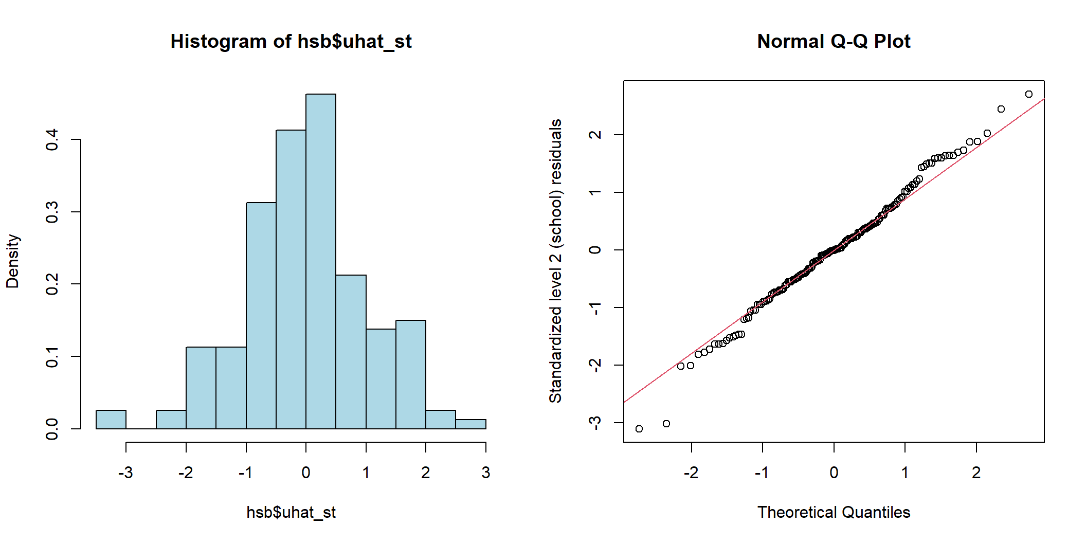
图 48.4: Histogram and Q-Q plot of cluster (school) level standardized residuals for the intercept
par(mfrow=c(1,2))
hist(hsb_selected$ehat, freq = FALSE, breaks = 38, col='lightblue')
qqnorm(hsb_selected$ehat,  ylab = "Standardized level 1 (pupil) residuals"); qqline(hsb_selected$ehat, col=2)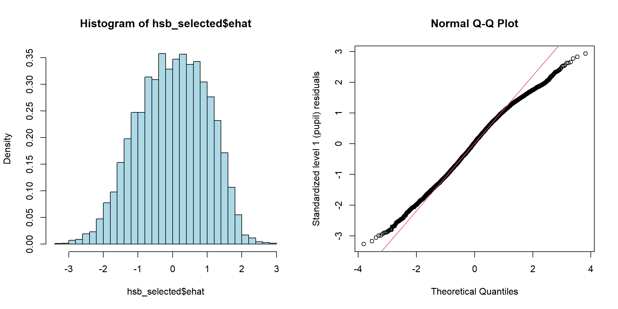
图 48.5: Histogram and Q-Q plot of individual (pupil) level standardized residuals for the intercept
48.8.10 通过刚刚所求的随机效应方差的残差,确认哪个学校存在相对极端的值。
# summ(hsb$uhat_st, graph = FALSE)
hsb %>%
  summarise(n = n(),
            mean_uhatst = mean(uhat_st),
            sd_uhatst = sd(uhat_st),
            min_uhatst = min(uhat_st),
            max_uhatst = max(uhat_st))
## n mean_uhatst sd_uhatst min_uhatst max_uhatst
## 1 160 -0.0007852687 1.006628 -3.107185 2.709731## sector mathach size uhat_st
## 48 1 13.874 687 2.709731## sector mathach size uhat_st
## 135 0 15.936 153 -3.018903
## 143 0 -2.081 745 -3.107185所以,此处可以看出,随机效应残差下提示的随机效应标准差可能比较极端的有上面这三所规模较小的学校。其中一所是天主教会学校,另外两所是非天主教会学校。
48.8.11 计算学校水平的 SES 平均值,以及每个学生自己和所在学校均值之间的差值大小。分别拟合两个不同的混合效应模型,一个只用 SES,另一个换做使用新计算的组均值和组内均差。
Mean_ses_math <- plyr::ddply(hsb_selected,~schoolid,summarise,mean_ses=mean(ses),mean_math=mean(mathach))


hsb_selected$dif_ses <- NA
for (i in Mean_ses_math$schoolid) {
hsb_selected$dif_ses[which(hsb_selected$schoolid == i)] <-  hsb_selected$ses[which(hsb_selected$schoolid == i)] -
  Mean_ses_math$mean_ses[which(Mean_ses_math$schoolid == i)]
}

hsb_selected <- hsb_selected %>%
  mutate(mean_ses = ses - dif_ses)

## total simple model with ses only
Simple_reml <- lmer(mathach ~ ses + (1 | schoolid), data = hsb_selected, REML = TRUE)
summary(Simple_reml)
## Linear mixed model fit by REML. t-tests use Satterthwaite's method [
## lmerModLmerTest]
## Formula: mathach ~ ses + (1 | schoolid)
## Data: hsb_selected
##
## REML criterion at convergence: 46645.2
##
## Scaled residuals:
## Min 1Q Median 3Q Max
## -3.12607 -0.72720 0.02188 0.75772 2.91912
##
## Random effects:
## Groups Name Variance Std.Dev.
## schoolid (Intercept) 4.768 2.184
## Residual 37.034 6.086
## Number of obs: 7185, groups: schoolid, 160
##
## Fixed effects:
## Estimate Std. Error df t value Pr(>|t|)
## (Intercept) 12.6575 0.1880 148.3022 67.33 <2e-16 ***
## ses 2.3902 0.1057 6838.0776 22.61 <2e-16 ***
## ---
## Signif. codes: 0 '***' 0.001 '**' 0.01 '*' 0.05 '.' 0.1 ' ' 1
##
## Correlation of Fixed Effects:
## (Intr)
## ses 0.003## fit the extended model within and between effect separated
Extend_reml <- lmer(mathach ~ dif_ses + mean_ses + (1 | schoolid), data = hsb_selected, REML = TRUE)
## the between schools effect (5.87) seems much larger than the within school effect (2.19)
summary(Extend_reml)## Linear mixed model fit by REML. t-tests use Satterthwaite's method [
## lmerModLmerTest]
## Formula: mathach ~ dif_ses + mean_ses + (1 | schoolid)
## Data: hsb_selected
##
## REML criterion at convergence: 46568.6
##
## Scaled residuals:
## Min 1Q Median 3Q Max
## -3.1666 -0.7254 0.0174 0.7558 2.9454
##
## Random effects:
## Groups Name Variance Std.Dev.
## schoolid (Intercept) 2.693 1.641
## Residual 37.019 6.084
## Number of obs: 7185, groups: schoolid, 160
##
## Fixed effects:
## Estimate Std. Error df t value Pr(>|t|)
## (Intercept) 12.6833 0.1494 153.6518 84.91 <2e-16 ***
## dif_ses 2.1912 0.1087 7021.5092 20.16 <2e-16 ***
## mean_ses 5.8662 0.3617 153.3666 16.22 <2e-16 ***
## ---
## Signif. codes: 0 '***' 0.001 '**' 0.01 '*' 0.05 '.' 0.1 ' ' 1
##
## Correlation of Fixed Effects:
## (Intr) dif_ss
## dif_ses 0.000
## mean_ses 0.010 0.000## We find strong evidence to support that the second model gives a better fit to the data
mod2<- update(Extend_reml, . ~ . - dif_ses - mean_ses)
anova(Extend_reml, mod2)## refitting model(s) with ML (instead of REML)## Data: hsb_selected
## Models:
## mod2: mathach ~ (1 | schoolid)
## Extend_reml: mathach ~ dif_ses + mean_ses + (1 | schoolid)
## npar AIC BIC logLik deviance Chisq Df Pr(>Chisq)
## mod2 3 47122 47142 -23558 47116
## Extend_reml 5 46574 46608 -23282 46564 552 2 < 2.2e-16 ***
## ---
## Signif. codes: 0 '***' 0.001 '**' 0.01 '*' 0.05 '.' 0.1 ' ' 1