第 32 章 排列置换法
32.1 背景介绍
Good(Good 2006) 曾经提出假设检验构建的步骤,这里引用如下:
- 分析问题,确认零假设 (null hypothesis),和可能的替代假设 (alternative hypothesis)。确认这两种假设决定以后可能伴随的错误 (The potential risk associated with a decision);
- 选择一个检验统计量;
- 计算数据给出的检验统计量;
- 确定检验统计量,在零假设时的样本分布;
- 用确定好的样本分布,以及数据给出的统计量大小,做出决策!
本章要介绍的排列置换法 (permutation),和下一章会介绍的自助重抽法 (bootstrap) ,需要大量的计算机的计算,和较强的电脑性能。这两种方法有一个共同的特征,它们都利用手头获得的样本数据辅助生成样本分布,同时对该数据的分布或者特质不进行假设。也就是用在上面罗列步骤的第4步。其余的步骤则与一般的参数假设检验完全相同。
32.2 直接上实例
之前用过的甲亢数据:
| thyr | group |
|---|---|
| 34 | Slight or no symptoms |
| 45 | Slight or no symptoms |
| 49 | Slight or no symptoms |
| 55 | Slight or no symptoms |
| 58 | Slight or no symptoms |
| 59 | Slight or no symptoms |
| 60 | Slight or no symptoms |
| 62 | Slight or no symptoms |
| 86 | Slight or no symptoms |
| 5 | Marked symptoms |
| 8 | Marked symptoms |
| 18 | Marked symptoms |
| 24 | Marked symptoms |
| 60 | Marked symptoms |
| 84 | Marked symptoms |
| 96 | Marked symptoms |
我们来计算这个数据中不同组的甲状腺素的平均值,标准差,中位数等特征描述量;
## For dt$group = Marked symptoms
##  obs. mean   median  s.d.   min.   max.
##  7    42.143 24      37.481 5      96
##
## For dt$group = Slight or no symptoms
##  obs. mean   median  s.d.   min.   max.
##  9    56.444 58      14.222 34     86
这个例子中我们关心的是,两组之间的甲状腺素水平是否相同。所以,我们的检验统计量在这里就可以定义为两组之间均值差,或者中位数差,我们先考虑用均值时的情况。
\[ T=\bar{Y}_1 - \bar{Y}_2 \] 接下来我们需要这个统计量 \(T\) 的样本分布,同时我们不对数据进行任何分布的假设 (数据不被认为是正态分布或者服从其他任何已知的分布)。
在排列置换法中,我们利用的原则是,在零假设的条件下,所有观察值的分组可以随机改变。也就是说,我们认为,零假设时,所有的观察数据,均来自于一个相同且未知的分布,每一个观察值的分组标签对平均值没有影响。故,此例中我们可以这样认为:
- 每个人的甲状腺激素水平相同,不受分组情况影响;
- 轻微或无症状组的人如果也在显著症状组,他们的甲状腺激素水平不会改变;
- 改变任何一个人的组别信息,对均值没有影响。
利用上述原则,检验统计量 \(T\) 的样本分布,就是所有16个人的组别信息的排列组合的情况下,观察值的均值差异大小。所以,我们可以对16个观察对象的组别信息随机分配,计算每一次分组情况下的观察值均值差,获得零假设条件下,检验统计量的样本分布。
这里使用 R 进行组别的随机分配:
#用 sample 对组别信息重新随机排列
set.seed(1234)
g1 <- sample(dt$group, length(dt$group), FALSE) # FALSE means replace = FALSE
g2 <- sample(dt$group, length(dt$group), FALSE)
g3 <- sample(dt$group, length(dt$group), FALSE)
g4 <- sample(dt$group, length(dt$group), FALSE)
g5 <- sample(dt$group, length(dt$group), FALSE)
dt <- cbind(dt, g1, g2, g3, g4, g5)
kable(dt, "html", align = "c",caption = "Serum thyroxine levels with permuted groups") %>%
  kable_styling(bootstrap_options = c("striped", "bordered")) %>%
scroll_box(width = "780px", height = "500px", extra_css="margin-left: auto; margin-right: auto;")| thyr | group | g1 | g2 | g3 | g4 | g5 |
|---|---|---|---|---|---|---|
| 34 | Slight or no symptoms | Marked symptoms | Marked symptoms | Marked symptoms | Slight or no symptoms | Slight or no symptoms |
| 45 | Slight or no symptoms | Marked symptoms | Marked symptoms | Slight or no symptoms | Slight or no symptoms | Slight or no symptoms |
| 49 | Slight or no symptoms | Slight or no symptoms | Slight or no symptoms | Marked symptoms | Marked symptoms | Slight or no symptoms |
| 55 | Slight or no symptoms | Slight or no symptoms | Slight or no symptoms | Slight or no symptoms | Slight or no symptoms | Marked symptoms |
| 58 | Slight or no symptoms | Marked symptoms | Marked symptoms | Marked symptoms | Slight or no symptoms | Marked symptoms |
| 59 | Slight or no symptoms | Slight or no symptoms | Slight or no symptoms | Slight or no symptoms | Marked symptoms | Marked symptoms |
| 60 | Slight or no symptoms | Marked symptoms | Marked symptoms | Slight or no symptoms | Marked symptoms | Marked symptoms |
| 62 | Slight or no symptoms | Marked symptoms | Marked symptoms | Slight or no symptoms | Marked symptoms | Slight or no symptoms |
| 86 | Slight or no symptoms | Slight or no symptoms | Marked symptoms | Marked symptoms | Slight or no symptoms | Marked symptoms |
| 5 | Marked symptoms | Slight or no symptoms | Slight or no symptoms | Slight or no symptoms | Slight or no symptoms | Slight or no symptoms |
| 8 | Marked symptoms | Slight or no symptoms | Slight or no symptoms | Marked symptoms | Marked symptoms | Slight or no symptoms |
| 18 | Marked symptoms | Marked symptoms | Marked symptoms | Slight or no symptoms | Marked symptoms | Marked symptoms |
| 24 | Marked symptoms | Marked symptoms | Slight or no symptoms | Marked symptoms | Slight or no symptoms | Marked symptoms |
| 60 | Marked symptoms | Slight or no symptoms | Slight or no symptoms | Slight or no symptoms | Slight or no symptoms | Slight or no symptoms |
| 84 | Marked symptoms | Slight or no symptoms | Slight or no symptoms | Slight or no symptoms | Slight or no symptoms | Slight or no symptoms |
| 96 | Marked symptoms | Slight or no symptoms | Slight or no symptoms | Marked symptoms | Marked symptoms | Slight or no symptoms |
接下来我们就可以计算当观察对象的组别信息不同时,检验统计量 \(T\) 的分布:
## [1] 14.301587## [1] 12.777778## [1] -2.968254## [1] -0.93650794## [1] -0.17460317## [1] -2.2063492所以理论上,我们可以把16人中任意7人陪分配到“轻微或无症状”组的所有排列组合穷举出来(有\(\binom{16}{7} = 11,440\) 不同的分组法),计算出所有情况下的均值差,组成我们感兴趣的统计量的样本分布。所以你会看到,当我们的样本量只有16个人的时候,两组分配已经达到上万种之多,样本量增加之后,计算量是成几何级倍数在增加的。例如20人中两组各10人的分组种类有:\(\binom{20}{10} = 184,756\) 种,30人中两组个15人的分组种类有:\(\binom{30}{15} = 1.55\times10^8\) 种之多。所以实际情况下,我们通常的解决办法是,随机从所有可能的分组法中抽出足够多的配列组合。下面以这个甲状腺数据为例,我们对11,440种可能的排列组合随机抽出10000种排列计算这10000个不同的均值差:
set.seed(1)
dist <- replicate(10000, t.test(sample(dt$thyr, length(dt$thyr), FALSE) ~ dt$group, var.equal = TRUE)$statistic)
上面的代码的涵义是从样本对观察值进行10000次排列组合,对每个组合进行 \(t\) 检验,获取 \(t\) 检验的统计量。下面把观察值原本的统计量的位置标记在所有10000次组合给出的统计量的柱状图中。
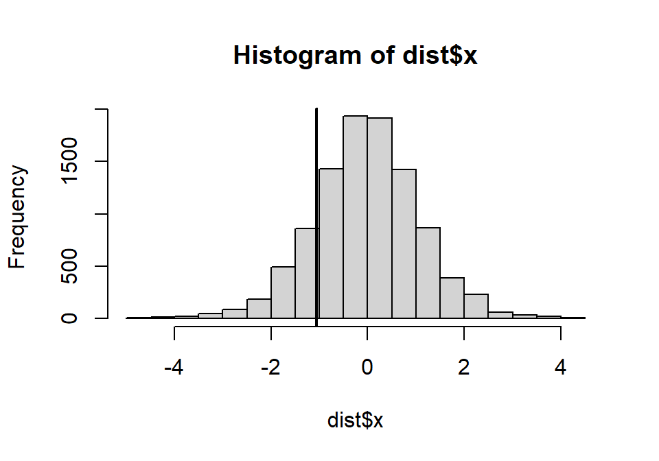
图 32.1: The sampling distribution of the difference
可以看出来,观察值的统计量在这10000个新样本中,并不那么“极端”。观察数据的排列置换法 \(p\) 值为:
#Use the distribution to obtain a p-value for the mean-difference by counting how many permuted mean-differences are more extreme than the one we observed in our actual data:
sum(abs(dist) > abs(t.test(dt$thyr ~ dt$group, var.equal = TRUE)$statistic))/10000
## [1] 0.3072跟下面用参数检验法的 \(p\) 值结果做一下对比,就会发现,其实二者的 \(p\) 值结果十分接近。
##
##  Two Sample t-test
##
## data:  dt$thyr by dt$group
## t = -1.05935, df = 14, p-value = 0.30738
## alternative hypothesis: true difference in means between group Marked symptoms and group Slight or no symptoms is not equal to 0
## 95 percent confidence interval:
##  -43.256997  14.653823
## sample estimates:
##       mean in group Marked symptoms mean in group Slight or no symptoms
##                           42.142857                           56.444444
32.3 排列置换法三板斧
标题党会不服,其实排列置换法的步骤不止三步 (笑)。
- 在零假设的前提下,确认观察数据所属的组别,是可以任意对调的。 (exchangeability) 有时候我们可能对数据进行一些转换 (transforming),以满足这个要求。
- 确认检验统计量 \(T\),用 \(T_{NULL}\) 标记。并且确定零假设时,检验统计量的期待值。 (通常会用 \(T_{NULL}=0\))
- 计算观察数据获得的统计量 \(T_0\)。
- 对观察对象的组别进行 \(N\) 次随机排列组合。计算每次排列组合情况下的统计量 \((T_1, T_2, \cdots, T_N)\)。
- 计算\((T_1, T_2, \cdots, T_N)\) 中比\(T_0\) 更极端的值所占的比例(\(>|T_0|\)),作为观察值\(T_0\) 的双侧\(p\) 值。
32.3.1 该如何选用合适的检验统计量 \(T\)?
在排列置换法中选用合适的检验统计量是一个需要仔细思考的过程。选用的 \(T\) 必须要能反映组间的差异,并且要与话题相关。也希望能够尽量和另假设时的统计量有一定的距离\(T_{NULL}\)。然而,选择了不同的检验统计量并不意味着统计结果会有天差地别。最终常常是殊途同归。另外,检验统计量并不一定要是一般参数检验时用到的统计量(\(t\) 或者其他的似然比检验),因为我们不需要对统计量的精确度(标准差标准误等统统不要)作判断,本法的统计学推断是通过排列置换的过程实现的。
32.3.2 可以在排列置换法中对其他变量进行统计学调整 (adjustment) 吗?
用随机对照试验做例子。假如在实验开始前的某个测量变量需要作为共变量被调整 (也就是要用 ANCOVA),以获得调整后的 \(Y\) 差异。在零假设条件下,\(Y_i\) 就不满足可置换原则 (exchangeable),因为那个需要被调整的测量变量可能决定了他们之间组别是有差异的。
此时,零假设条件 (没有组间差异) 下,满足可置换原则的其实是不考虑组别的情况下对需要校正的变量进行线性回归后获得的残差 \(R_i\):
\[ R_i = Y_i - \hat{Y}_i = Y_i - \hat\alpha - \hat\beta X_i \]
另假设条件下,只有残差 \(R_i\) 才满足可置换原则,可以用在排列置换法中。当需要调整的变量个数增加时,同样适用。
32.3.3 排列置换法,基于秩次的非参数检验之间的关系
如果你注意到,当我们把原始观察数据排序之后进行的排序检验其实就是我们本章介绍的排列置换法。它在前面的秩次非参数检验中以特殊的形式展现。 Good (Good 2006) 曾经说的好,“99% of common non-parametric tests are permutation tests in which the observations have been replaced by ranks. The sign is one notable exception.” 所以符号检验是非排序检验的特例。
32.3.4 排列置换检验法,是一种精确检验
复合型假设,指的是假设中只提及了所有分布情况中的一种的例如:
\[\text{The mean of X is equal to } 0\]
相反,一个简单假设,则是对参数分布进行了详细描述的假设:
\[X\sim N(0,4)\]
所以,对复合型假设进行的统计检验法,被称作精确检验法。精确检验法的特点是,复合型假设中包含的所有假设发生的概率之和等于该检验法的第一类错误概率 \(\alpha\)。
A test is said to be exact with respect to a compound hypothesis if the probability of making a type I error is exactly \(\alpha\) for each and every one of the simple hypotheses that are subsumed within the compound hypothesis.
一个大家都听说过的精确检验的例子就是 Fisher 精确检验法 (也是一种排列置换检验)。 所有的排列置换检验法都是精确检验法。
32.4 基于排序置换检验法计算置信区间
基于排序置换检验法的置信区间计算,是一个有些许繁琐的过程。我们可以设定多个不同的 \(N_{NULL}\) ,但是样本分布相同的零假设时的统计量。计算相应的 \(p\) 值,95% 置信区间就是 \(p\) 值保持大于等于 \(0.05\)的 \(N_{NULL}\) 取值范围。计算量将会是很大的。
用前面的例子来解释就是,我们可以假设两组之间甲状腺素的差异是\(T_{NULL} = 10\),然后将第二组的观察值全部加上10 (或者将第一组的观察值全部减去10),然后用前面描述的方法来检验两组之间的差是否等于零,获取\(p\) 值。然后用不同的 \(T_{NULL}\) 取值,重复这个过程,直到找到上限和下限的 \(T_{NULL}\) 值,他们的检验 \(p\) 值都是0.05。