第 34 章 广义线性回归入门
线性回归方法是十分强大的建模工具,可惜的是它只能适用与因变量为连续型变量的情况。广义线性回归模型 (或者叫一般化线性回归模型 generalised linear models, GLM) 是一大类将线性回归模型拓展到因变量可以使用二进制,计数,分组型变量的建模工具。
34.1 指数分布家族
一个服从正态分布的随机变量 \(Y\) 的概率密度方程 (probability density function, PDF) 可以写作
\[ f(y) = \frac{1}{\sqrt{2\pi\sigma^2}}e^{-\frac{(y-\mu)^2}{2\sigma^2}} \]
给 PDF 的左右两边同时取自然底数的对数,方程变形为
\[ \begin{aligned} \text{ln}\{f(y)\} & = -\frac{y^2}{2\sigma^2} + \frac{y\cdot\mu}{\sigma^2} - \frac{ \mu^2}{2\sigma^2} -\frac{1}{2}\text{ln}(2\pi\sigma^2) \\ & = \frac{y\cdot\mu - \frac{\mu^2}{2}}{\sigma^2} - [\frac{y^2}{2\sigma^2} + \frac{1 }{2}\text{ln}(2\pi\sigma^2) ] \end{aligned} \tag{34.1} \]
如果令
\[ \begin{aligned} \theta & = \mu \\ \psi & = \sigma^2 \\ b(\theta) & = \frac{\mu^2}{2} \\ c(y, \theta) & = \frac{y^2}{2\sigma^2} + \frac{1}{2}\text{ln}(2\pi\sigma^2) \end{aligned} \]
那么上面的式子 (34.1) 可以被整理为:
\[ \begin{equation} \text{ln}\{f(y)\} = \frac{y\cdot\theta - b(\theta)}{\psi} - c(y, \theta) \end{equation} \tag{34.2} \]
此处有重要结论: 凡是分布的概率密度方程的对数方程能够转换整理成(34.2) 形式的分布,都隶属于指数分布家族(the Exponential Family of distributions) 。
34.1.1 泊松分布和二项分布的指数分布家族属性
- 泊松分布 Poisson Distribution
\[ \begin{aligned} f(y) & = \text{Pr}(Y = y) = \frac{\mu^y e^{-\mu}}{y!}, y = 0,1,2,\cdots \\ \text{ln}\{ f(y) \} & = y\cdot\text{ln}(\mu) - \mu - \text{ln}(y!) \\ \text{Let } &\color{red}{\boxed{\theta = \text{ln}(\mu), \psi = 1, b(\theta) = \mu, c(y,\psi) = \text{ln}(y!)}} \\ \Rightarrow \text{ln}\{f(y)\} & = \frac{y\cdot\theta - b(\theta)}{\psi} - c(y, \theta) \\ \end{aligned} \]
所以,泊松分布属于指数分布家族成员。
- 二项分布 Binommial Distribution
\[ \begin{aligned} f(y) & = \text{Pr}(Y = y) = \binom{n}{y}\pi^y(1-\pi)^{n-y}, y = 0,1,2,\cdots \\ \text{ln}\{ f(y) \} & = y\cdot \text{ln}(\pi) + (n - y)\text{ln}(1-\pi) + \text{ln} \{\binom{n}{y}\} \\ & = y\cdot \text{ln}(\frac{\pi}{1-\pi}) + n\text{ln}(1-\pi) + \text{ln}\{\binom{n} {y}\} \\ \text{Let } &\color{red}{\boxed{\theta = \text{ln}(\frac{\pi}{1-\pi}), \psi = 1,}} \\ &\color{red}{\boxed{b(\theta) = -n\text{ln}(1-\pi), c(y, \psi) = -\text{ln}\{\binom{n }{y}\}}}\\ \Rightarrow \text{ln}\{f(y)\} & = \frac{y\cdot\theta - b(\theta)}{\psi} - c(y, \theta) \\ \end{aligned} \]
所以,二项分布也属于指数分布家族成员。
指数分布家族成员的数学表达式 (34.2) 中,
- \(\theta\) 被叫做标准(或者叫自然) 参数(canonical or natural parameter),相关的函数被叫做标准链接函数(canonical link function),如上面所列举的例子中:泊松分布时用的对数函数\(\text{ln}(\mu)\),二项分布时用的逻辑函数(logit function) \(\text{ln}(\frac{\pi}{1-\pi})\) ,链接函数可能还有别的选择,(例如,二项分布数据的另一种标准链接函数是概率函数(probit function \(\Phi^{-1}(P)\))),同时它对于条件推断conditional inference 至关重要,因为它还提示我们应该用什么样的算法去估计我们苦苦寻找的人群参数。
- \(\phi\) 被命名为尺度参数 (scale or dispersion parameter),泊松分布和二项分布的尺度参数是 \(1\)。但是正态分布的尺度参数是方差 \(\sigma^2\),且常常是未知的,需要从样本数据中估计。尺度参数是否需要从样本中获取其估计值,对于实际统计推断或者假设检验的过程有重大影响。
广义线性回归就是这个指数分布家族数据共通的一种统计建模过程,所以,在这一“屋檐”下,它衍生出众多种类的统计模型。
34.1.2 Exercise. Exponential distribution
证明指数分布本身也属于指数分布家族,定义其标准链接函数和标准参数。
证明
\[ \begin{aligned} Y \sim \text{exp}(\lambda) & \rightarrow f(y) = \lambda \text{exp}(-y\lambda), y > 0\\ \Rightarrow \text{ln}\{ f(y) \} & = - y \lambda + \text{ln}(\lambda) \\ \text{Let } & \color{red}{\theta = -\lambda, b(\theta) = - \text{ln}(\lambda), \phi = 1, c(y, \phi) = 0 } \\ \Rightarrow \text{ln}\{f(y)\} & = \frac{y\cdot\theta - b(\theta)}{\phi} - c(y, \theta) \\ \text{Because } E(Y) & = \frac{1}{\lambda}, \text{ the canonical link is } g(\lambda) = -\frac{1}{\lambda}\\ \end{aligned} \]
34.2 广义线性回归模型之定义
一个四肢健全的广义线性模型包括三个部分:
- 因变量分布(或者叫响应变量分布,response distribution):\(Y_i, i = 1,\cdots,n\) 可以被认为是互相独立且服从指数家族分布,设其期望值(均值) \(E( Y_i) = \mu_i\);
- 线性预测方程(linear predictor):预测变量及其各自的参数以线性回归形式进入模型,其中第\(i\) 个观测值的线性预测值为:
\[\eta_i = \alpha + \beta_1 x_{i1} + \cdots + \beta_p x_{ip}\] - 链接函数 (link function):链接函数连接的是线性预测方程 \(\eta_i\) 和其期待值 (均值) 之间 \(\mu_i\) 的关系。
\[g(\mu_i) = \eta_i\]
简单线性回归模型本身当然也数据广义线性回归模型:
- 因变量分布是正态分布;
- 线性预测值也是线性回归形式;
- 链接函数是它因变量本身 (the identity function)。
34.3 注意
- 广义线性回归的线性预测方程部分的意义,需要澄清的是它指的是参数parameter 之间呈线性关系,预测变量本身可以有二次方,三次方,多次方,因为这些多项式线性回归本身仍然是线性的如: \[\eta_i = \alpha + \beta_1 x_i + \beta_2 x_i^2 + \cdots + \beta_p x_i^p\]
然而,这样的形式\[\eta_i = \alpha (1- e^{\beta_1 x_{i1}})\]
就不能说是一个线性预测方程。 - 除了有很少的特例。广义线性回归拟合后的参数估计,推断,模型评价和比较时使用的原理都一样,不同的只有各自的分布和链接函数。
- 通常选用的链接方程,要能够使线性预测方程的取值范围达到所有实数 \(-\infty,+\infty\)。
- “模型的似然函数the log likelihood of the model”,只是我们偷懒缩短了原文“在给定数据的前提下,当所有参数均为\(\text{MLE}\) 时模型的对数似然函数(the log likelihood function of the model for the given data evaluated at the MLE’s of the parameters)”,就是对数似然函数的极大值的意思(i.e. the maximum of the log likelihood function)。
- 从本节开始往后的章节中 “模型,model”,“广义线性模型,generalized linear model”,和 “GLM” 将被视为同义词。
34.4 如何在 R 里拟合 “GLM”
这里讨论用极大似然法拟合 “GLM” 模型的方法。前面一章节的复习也是在告诉我们,利用极大似然法简单说就是找到模型参数,使得似然函数能够取到极大值。对于线性回归来说, \(\text{MLE}\) 可以用一个封闭式函数来计算;但是广义线性回归模型则必须使用迭代法计算(iterative methods)。
在 R 里面拟合广义线性模型的命令及其格式是:
glm(response variable ~ explanatory variables to form linear predictor, family=name of distribution(link=link function), data=dataset)Tips: See help(glm) for other modeling options. See help(family) for other allowable link functions for each family.
下面的数据来自一个心理学临床实验,比较的是和安慰剂组相比,注射吗啡组,注射海洛因组对象的精神病检测指数的前后变化。
Mental <- read.table("../backupfiles/MENTAL.DAT", header =  FALSE, sep ="", col.names = c("treatment", "Before", "After"))
Mental$treatment[Mental$treatment == 1] <- "placebo"
Mental$treatment[Mental$treatment == 2] <- "morphine"
Mental$treatment[Mental$treatment == 3] <- "heroin"
Mental$treatment <- factor(Mental$treatment, levels = c("placebo", "morphine", "heroin"))
head(Mental)
## treatment Before After
## 1 placebo 0 7
## 2 placebo 2 1
## 3 placebo 14 10
## 4 placebo 5 10
## 5 placebo 5 6
## 6 placebo 4 2我们来比较一下简单线性回归的代码输出结果和广义线性回归代码输出结果是否一致:
用 lm 命令,拟合因变量为注射后精神病检测指数,预测变量为治疗方式和注射钱精神病检测指数,及两者的交互作用项:
##
## Call:
## lm(formula = After ~ treatment * Before, data = Mental)
##
## Residuals:
##     Min      1Q  Median      3Q     Max
## -7.8281 -1.9351 -0.5161  1.4161 11.3601
##
## Coefficients:
##                          Estimate Std. Error t value Pr(>|t|)
## (Intercept)               1.97803    1.29407   1.529  0.13116
## treatmentmorphine        -1.21174    1.75034  -0.692  0.49118
## treatmentheroin          -1.46197    1.77186  -0.825  0.41228
## Before                    0.59394    0.18347   3.237  0.00189 **
## treatmentmorphine:Before -0.08953    0.24835  -0.360  0.71963
## treatmentheroin:Before   -0.31299    0.25038  -1.250  0.21570
## ---
## Signif. codes:  0 '***' 0.001 '**' 0.01 '*' 0.05 '.' 0.1 ' ' 1
##
## Residual standard error: 3.333 on 66 degrees of freedom
## Multiple R-squared:  0.3442, Adjusted R-squared:  0.2945
## F-statistic: 6.927 on 5 and 66 DF,  p-value: 2.974e-05
同样的模型也可以用 glm 命令拟合:
Model2 <- glm(After ~ treatment*Before, family = gaussian(link = "identity"), data = Mental)
summary(Model2)
##
## Call:
## glm(formula = After ~ treatment * Before, family = gaussian(link = "identity"),
## data = Mental)
##
## Coefficients:
## Estimate Std. Error t value Pr(>|t|)
## (Intercept) 1.97803 1.29407 1.529 0.13116
## treatmentmorphine -1.21174 1.75034 -0.692 0.49118
## treatmentheroin -1.46197 1.77186 -0.825 0.41228
## Before 0.59394 0.18347 3.237 0.00189 **
## treatmentmorphine:Before -0.08953 0.24835 -0.360 0.71963
## treatmentheroin:Before -0.31299 0.25038 -1.250 0.21570
## ---
## Signif. codes: 0 '***' 0.001 '**' 0.01 '*' 0.05 '.' 0.1 ' ' 1
##
## (Dispersion parameter for gaussian family taken to be 11.10799)
##
## Null deviance: 1117.88 on 71 degrees of freedom
## Residual deviance: 733.13 on 66 degrees of freedom
## AIC: 385.41
##
## Number of Fisher Scoring iterations: 2可以用下面的各种命令获取想要的各种有用的信息
##                               2.5 %    97.5 %
## (Intercept)              -0.5582981 4.5143587
## treatmentmorphine        -4.6423492 2.2188654
## treatmentheroin          -4.9347406 2.0108045
## Before                    0.2343483 0.9535305
## treatmentmorphine:Before -0.5762749 0.3972233
## treatmentheroin:Before -0.8037270 0.1777561## (Intercept) treatmentmorphine treatmentheroin
## 7.2284910 0.2976783 0.2317797
## Before treatmentmorphine:Before treatmentheroin:Before
## 1.8111091 0.9143647 0.7312605## 2.5 % 97.5 %
## (Intercept) 0.572182041 91.318984
## treatmentmorphine 0.009635036 9.196890
## treatmentheroin 0.007192327 7.469324
## Before 1.264084682 2.594855
## treatmentmorphine:Before 0.561987950 1.487688
## treatmentheroin:Before 0.447657446 1.194534## 1 2 3 4 5 6
## 1.978030 3.165909 10.293182 4.947727 4.947727 4.353788## 1 2 3 4 5 6
## 5.0219697 -2.1659091 -0.2931818 5.0522727 1.0522727 -2.353787934.4.1 margins 命令
一个在 STATA 里面十分有用的用于预测的命令 margins,在 R 里,下载了 margins 包以后就可以调用和 STATA 的 margins 类似的命令。
假如我们用拟合的模型预测当注射前精神病检测值分别是 0,6,12 分时三组之间的注射后精神病检测值差,可以这样求:
##             factor  Before     AME     SE       z      p   lower   upper
##             Before  0.0000  0.4598 0.1004  4.5797 0.0000  0.2630  0.6565
##             Before  6.0000  0.4598 0.1004  4.5797 0.0000  0.2630  0.6565
##             Before 12.0000  0.4598 0.1004  4.5797 0.0000  0.2630  0.6565
##    treatmentheroin  0.0000 -1.4620 1.7719 -0.8251 0.4093 -4.9347  2.0108
##    treatmentheroin  6.0000 -3.3399 0.9624 -3.4705 0.0005 -5.2261 -1.4537
##    treatmentheroin 12.0000 -5.2178 1.7963 -2.9048 0.0037 -8.7384 -1.6972
##  treatmentmorphine  0.0000 -1.2117 1.7503 -0.6923 0.4888 -4.6423  2.2189
##  treatmentmorphine  6.0000 -1.7489 0.9630 -1.8160 0.0694 -3.6364  0.1386
##  treatmentmorphine 12.0000 -2.2861 1.7977 -1.2716 0.2035 -5.8095  1.2374
34.4.2 ggplot2::geom_smooth(method = "loess") 命令
类似 STATA 作散点图时的 lowess 命令,在 R 里,你可以用 ggplot2 包里自带的 geom_smooth(method = "loess") 选项命令,给散点图添加平滑曲线。把观测数据中变量之间的关系视觉化,用于辅助判断一个模型是否可以被拟合为线性关系。全称是 “locally weighted scatterplot smoothing”,缩写成 “lowess/loess”。 LOWESS 的原理简略说是,通过把预测变量分成几个部分,分别在各个小区间内拟合回归各自的回归曲线,如此便可以将每个观测值都以各自不同的加权值放入整个模型中,然而正如我们在简单线性模型中提到过的,这样的曲线更加拟合观测数据,而不能说明观测值来自的人群中,两个变量之间的关系。此方法的灵活性在于,你可以选择平滑的程度,该平滑程度用bandwith(STATA) 或者span(R) 表示,取值范围是\(0 \sim 1\) 之间的任意值,越靠近\(1\),Lowess 曲线越接近简单线性直线,越靠近\(0\),那么每个观测点本身的权重越大,拟合的Lowess 曲线越接近观测数据本身。下图 34.1 提示,选用的平滑程度 \(= 0.8\) 时,精神病测量分数在 (安慰剂组中) 实验前后的关系接近线性关系。当我们降低平滑程度,Lowess 曲线接近观测数据本身,其实是太接近观测数据本身,反而无法提供太多的信息。
library(ggplot2)
ggplot(Mental, aes(Before, After)) + geom_point() +
  geom_smooth(method = "loess",  span = 0.8, se = FALSE) +
  facet_grid(treatment ~ .) + theme_bw()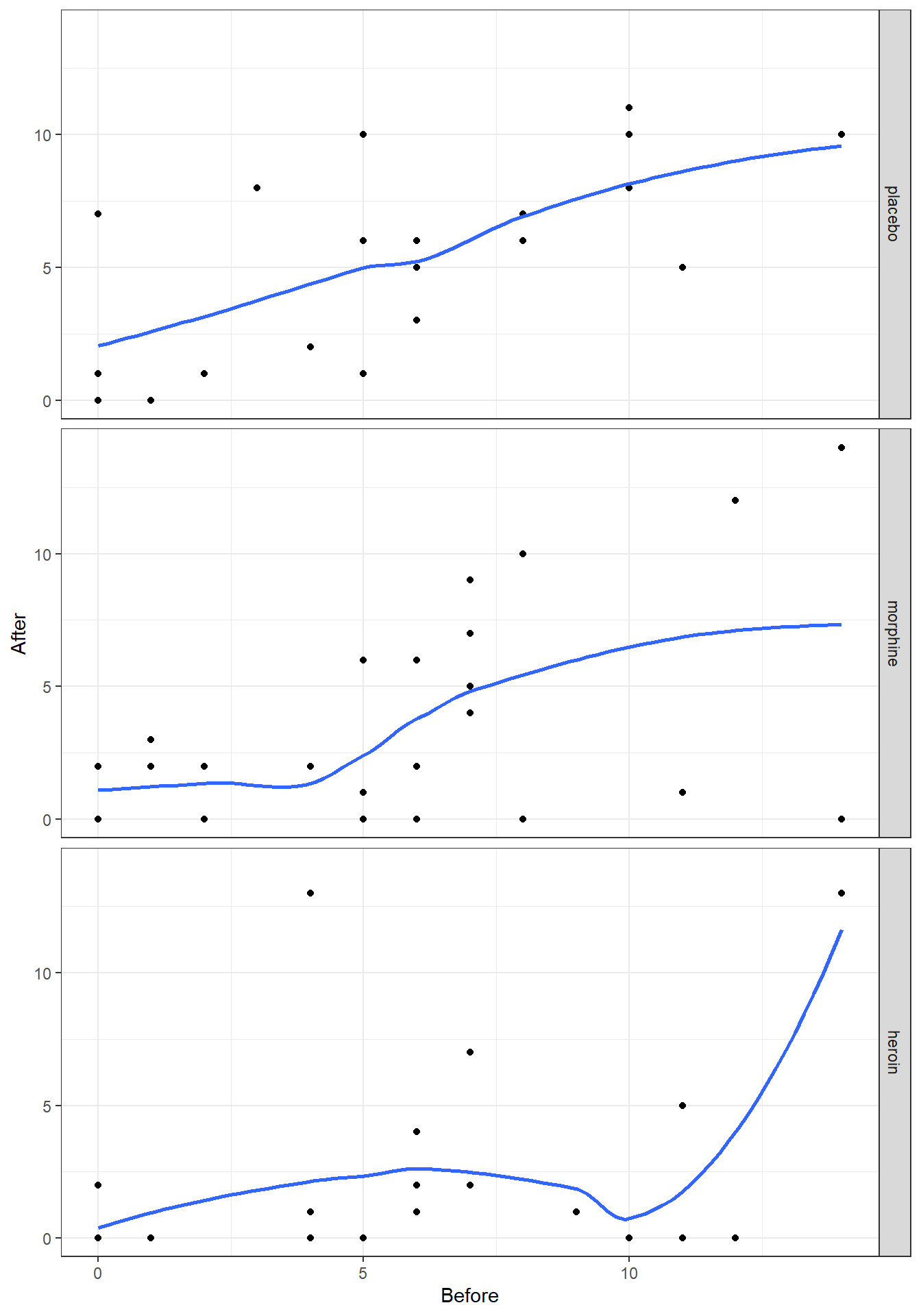
图 34.1: Lowess smoother, with bandwith/span set to 0.8, for the mental data
ggplot(Mental, aes(Before, After)) + geom_point() +
  geom_smooth(method = "loess",  span = 0.4, se = FALSE) +
  facet_grid(treatment ~ .) + theme_bw()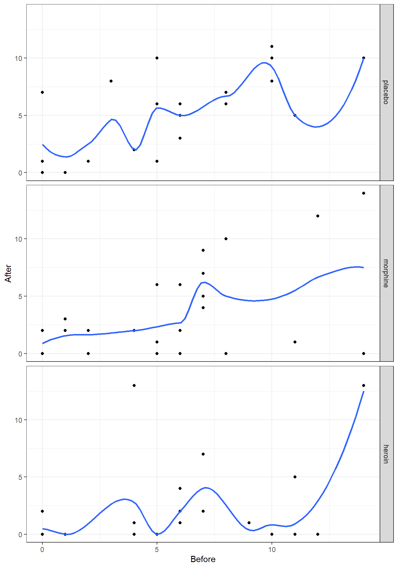
图 34.2: Lowess smoother, with bandwith/span set to 0.4, for the mental data
34.5 GLM例2
34.5.1 思考本章中指数分布家族的参数设置。假如,有一个观测值 \(y\) 来自指数家族。试求证:
MLE \(\hat\theta\) 是 \(b^\prime(\theta) = y\) 的解;
\(\theta\) 的 MLE 的方差是 \(\frac{\phi}{b^{\prime\prime}(\theta)}\);
如果\(Y\sim N(\mu, \sigma^2)\),试进一步证明\(b^\prime(\theta) = \mu\) 且\(\frac{\phi}{b^{\prime\ prime}(\theta)} = \sigma^2\)
当数据来自指数分布家族,它的对数似然可以写作:
\[ \frac{y\cdot\theta - b(\theta)}{\phi} - c(y, \phi) \]
对这个对数似然方程取 \(\theta\) 的偏微分方程可得:
\[ \frac{\partial}{\partial\theta}\ell(\theta,\phi) = \frac{y - b^\prime(\theta)}{\phi} \]
令此偏微分方程等于零,那么我们可以知道 \(\hat\theta\) 是 \(b^\prime(\theta) = y\) 的解。
- MLE 的方差可以用 Fisher information 来推导。
\[ S^2=\left.-\frac{1}{\ell^{\prime\prime}(\theta)}\right\vert_{\theta=\hat{\theta}} \\ \text{Because } \ell^{\prime\prime}(\theta) = -\frac{b^{\prime\prime}(\theta)}{\phi} \\ \Rightarrow S^2 = \frac{\phi}{b^{\prime\prime}(\theta)} \]
- 如果 \(Y\sim N(\mu, \sigma^2)\), 那么,根据正态分布数据属于指数家族的性质,
\[ \phi = \sigma^2,\theta = \mu, b(\theta =\mu) = \frac{\mu^2}{2} \\ \Rightarrow b^\prime(\theta) = \mu \\ \Rightarrow S^2 = \frac{\phi}{b^{\prime\prime}(\theta)} = \sigma^2 \]
34.5.2 R 练习
数据来自一个RCT临床试验,比较吗啡,海洛因和安慰剂在患者精神状态评分上的影响,试分析数据回答下面的问题:
- 三组治疗组之间注射后的评分均值不同吗?
- 调整基线时精神状态评分对你的模型结果有什么影响?
- 基线时精神状态评分的高低会影响不同药物的效果吗?
34.5.2.1 数据读入 R,作初步分析
Mental <- read.table("../backupfiles/MENTAL.DAT", header =  FALSE, sep ="", col.names = c("treatment", "prement", "mentact"))
Mental$treatment[Mental$treatment == 1] <- "placebo"
Mental$treatment[Mental$treatment == 2] <- "morphine"
Mental$treatment[Mental$treatment == 3] <- "heroin"
Mental$treatment <- factor(Mental$treatment, levels = c("placebo", "morphine", "heroin"))
head(Mental)
## treatment prement mentact
## 1 placebo 0 7
## 2 placebo 2 1
## 3 placebo 14 10
## 4 placebo 5 10
## 5 placebo 5 6
## 6 placebo 4 2library(ggplot2)
library(gridExtra)
# Use hsitograms and plots to look at the distributions of the pre- and post- injection scores.
# with(Mental, hist(prement, breaks = 14, freq = F))
# qplot(prement, data = Mental, binwidth = 1)
hist1 <- ggplot(Mental, aes(x = prement, y = after_stat(density))) + geom_histogram(binwidth = 1) + theme_bw()
hist2 <- ggplot(Mental, aes(x = mentact, y = after_stat(density))) + geom_histogram(binwidth = 1) + theme_bw()
Scatter <- ggplot(Mental, aes(x = prement, y = mentact)) + geom_point()+ theme_bw()
grid.arrange(hist1, hist2, Scatter, ncol=2)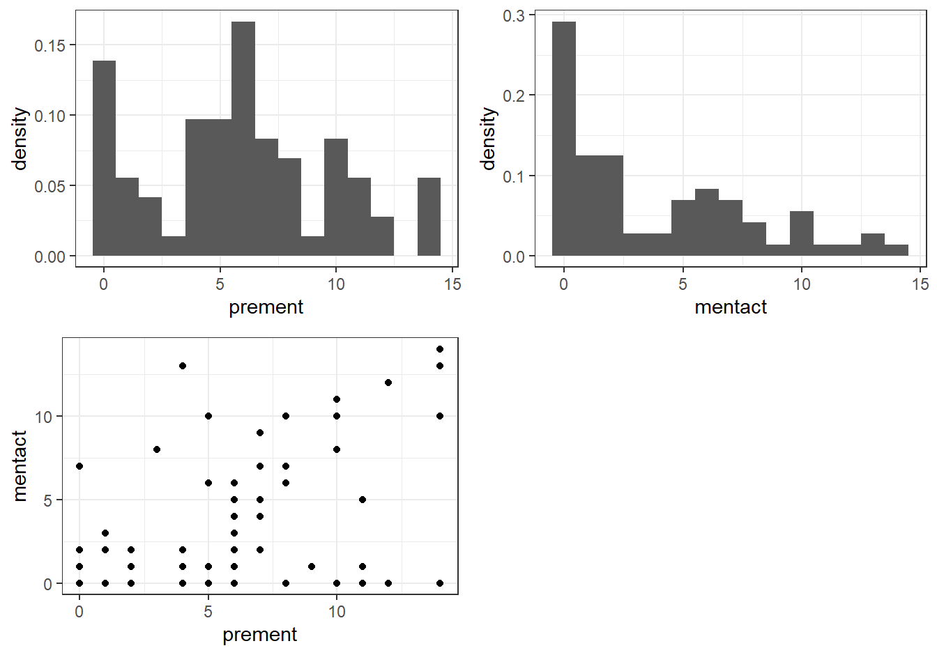
图 34.3: Histogram and plots
可以看到柱状图暗示我们实验前后的得分本身都不服从正态分布。但是这并不妨碍我们使用回归模型来做推断。毕竟,线性回归模型只要求残差服从正态分布。另外,散点图提示实验前后的得分之间可能呈正相关。
ggplot(Mental, aes(prement, mentact)) + geom_point() +
  geom_smooth(method = "loess",  span = 0.8, se = FALSE) +
  facet_grid(treatment ~ .) + theme_bw()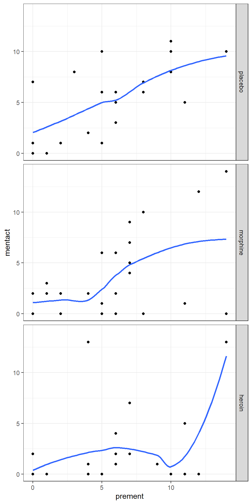
图 34.4: Lowess smoother, with bandwith/span set to 0.8, for the mental data
对于每组实验组来说,观测值数量都很少,姑且可以认为线性模型是合理的。
| Terms fitted | RSS | Residuals df |
|---|---|---|
|
1117.875 | 71 |
|
980.625 | 69 |
|
884.328 | 70 |
|
752.055 | 68 |
|
733.127 | 66 |
34.5.2.2 写下表格34.1 中五个线性回归模型的数学表达式,在R 里面拟合这5个模型,在第二列第三列分别填写各模型的统计信息(残差平方和residuals sum of squares,和残差自由度reiduals degrees of freedom)。利用该表格填写完整以后的内容,用笔和纸正式地比较模型 3 和 4; 4 和 5 的拟合优度。然后和 R 的输出结果比较确认。你会作出怎样的结论?另外,为什么相似的比较模型的方法不适用于比较模型 2 和 3?
解
用 \(z_i, y_i\) 分别标记第 \(i\) 名患者在药物注射前,后两次测量的精神医学指征评分。使用线性回归模型的前提假设是 \(y_i \sim N(\mu_i, \sigma^2)\) 且互相独立。另外,预测变量的标记为:
\[ x_{1i} = \left\{ \begin{array}{ll} 0 \text{ placebo or heroin }\\ 1 \text{ morphine}\\ \end{array} \right. x_{2i} = \left\{ \begin{array}{ll} 0 \text{ placebo or morphine }\\ 1 \text{ heroin}\\ \end{array} \right. \\ \]
- Overall mean model
链接方程部分: \(\eta_i = \beta_0\)
##
## Call:
## lm(formula = mentact ~ 1, data = Mental)
##
## Residuals:
##    Min     1Q Median     3Q    Max
## -3.792 -3.792 -1.792  2.458 10.208
##
## Coefficients:
##             Estimate Std. Error t value Pr(>|t|)
## (Intercept)   3.7917     0.4676   8.108 1.05e-11 ***
## ---
## Signif. codes:  0 '***' 0.001 '**' 0.01 '*' 0.05 '.' 0.1 ' ' 1
##
## Residual standard error: 3.968 on 71 degrees of freedom## Analysis of Variance Table
##
## Response: mentact
## Df Sum Sq Mean Sq F value Pr(>F)
## Residuals 71 1117.9 15.745- Drugs model
链接方程部分: \(\eta_i = \beta_0 + \beta_1 x_{1i} + \beta_2 x_{2i}\)
##
## Call:
## lm(formula = mentact ~ treatment, data = Mental)
##
## Residuals:
##    Min     1Q Median     3Q    Max
## -5.542 -2.167 -1.167  1.958 10.833
##
## Coefficients:
##                   Estimate Std. Error t value Pr(>|t|)
## (Intercept)         5.5417     0.7695   7.201 5.73e-10 ***
## treatmentmorphine  -1.8750     1.0883  -1.723  0.08938 .
## treatmentheroin    -3.3750     1.0883  -3.101  0.00279 **
## ---
## Signif. codes:  0 '***' 0.001 '**' 0.01 '*' 0.05 '.' 0.1 ' ' 1
##
## Residual standard error: 3.77 on 69 degrees of freedom
## Multiple R-squared:  0.1228, Adjusted R-squared:  0.09735
## F-statistic: 4.829 on 2 and 69 DF, p-value: 0.0109## Analysis of Variance Table
##
## Response: mentact
## Df Sum Sq Mean Sq F value Pr(>F)
## treatment 2 137.25 68.625 4.8287 0.0109 *
## Residuals 69 980.62 14.212
## ---
## Signif. codes: 0 '***' 0.001 '**' 0.01 '*' 0.05 '.' 0.1 ' ' 1- Pre-inj model
链接方程部分 \(\eta_i = \beta_0 + \beta_3z_i\)
##
## Call:
## lm(formula = mentact ~ prement, data = Mental)
##
## Residuals:
##     Min      1Q  Median      3Q     Max
## -7.5188 -2.3284 -0.8903  2.2542 10.0684
##
## Coefficients:
##             Estimate Std. Error t value Pr(>|t|)
## (Intercept)   1.0967     0.7539   1.455     0.15
## prement       0.4587     0.1067   4.300 5.43e-05 ***
## ---
## Signif. codes:  0 '***' 0.001 '**' 0.01 '*' 0.05 '.' 0.1 ' ' 1
##
## Residual standard error: 3.554 on 70 degrees of freedom
## Multiple R-squared:  0.2089, Adjusted R-squared:  0.1976
## F-statistic: 18.49 on 1 and 70 DF, p-value: 5.433e-05## Analysis of Variance Table
##
## Response: mentact
## Df Sum Sq Mean Sq F value Pr(>F)
## prement 1 233.55 233.547 18.487 5.433e-05 ***
## Residuals 70 884.33 12.633
## ---
## Signif. codes: 0 '***' 0.001 '**' 0.01 '*' 0.05 '.' 0.1 ' ' 1- Drugs + pre-inj model
链接方程部分: \(\eta_i = \beta_0 + \beta_1 x_{1i} + \beta_2 x_{2i} + \beta_3z_i\)
#4.  Drugs + Pre-inj model
Drug_Pre_inj <- lm(mentact ~ treatment + prement, data = Mental)
summary(Drug_Pre_inj)
##
## Call:
## lm(formula = mentact ~ treatment + prement, data = Mental)
##
## Residuals:
## Min 1Q Median 3Q Max
## -7.4118 -2.0548 -0.2288 1.0801 11.6845
##
## Coefficients:
## Estimate Std. Error t value Pr(>|t|)
## (Intercept) 2.81790 0.90542 3.112 0.002715 **
## treatmentmorphine -1.76151 0.96034 -1.834 0.070992 .
## treatmentheroin -3.31825 0.96010 -3.456 0.000949 ***
## prement 0.45396 0.09986 4.546 2.31e-05 ***
## ---
## Signif. codes: 0 '***' 0.001 '**' 0.01 '*' 0.05 '.' 0.1 ' ' 1
##
## Residual standard error: 3.326 on 68 degrees of freedom
## Multiple R-squared: 0.3272, Adjusted R-squared: 0.2976
## F-statistic: 11.03 on 3 and 68 DF, p-value: 5.492e-06## Analysis of Variance Table
##
## Response: mentact
## Df Sum Sq Mean Sq F value Pr(>F)
## treatment 2 137.25 68.625 6.205 0.003348 **
## prement 1 228.57 228.570 20.667 2.308e-05 ***
## Residuals 68 752.06 11.060
## ---
## Signif. codes: 0 '***' 0.001 '**' 0.01 '*' 0.05 '.' 0.1 ' ' 1- Drug + Pre-inj + Drug×Pre-inj
链接方程部分: $i = 0 + 1 x{1i} + 2 x{2i} + 3 z_i + {13}x{1i}z_i + {23}x_{2i}z_i $
#5.  Drugs + Pre-inj + Drug×Pre-inj model
Model5 <- lm(mentact ~ treatment*prement, data = Mental)
summary(Model5)
##
## Call:
## lm(formula = mentact ~ treatment * prement, data = Mental)
##
## Residuals:
## Min 1Q Median 3Q Max
## -7.8281 -1.9351 -0.5161 1.4161 11.3601
##
## Coefficients:
## Estimate Std. Error t value Pr(>|t|)
## (Intercept) 1.97803 1.29407 1.529 0.13116
## treatmentmorphine -1.21174 1.75034 -0.692 0.49118
## treatmentheroin -1.46197 1.77186 -0.825 0.41228
## prement 0.59394 0.18347 3.237 0.00189 **
## treatmentmorphine:prement -0.08953 0.24835 -0.360 0.71963
## treatmentheroin:prement -0.31299 0.25038 -1.250 0.21570
## ---
## Signif. codes: 0 '***' 0.001 '**' 0.01 '*' 0.05 '.' 0.1 ' ' 1
##
## Residual standard error: 3.333 on 66 degrees of freedom
## Multiple R-squared: 0.3442, Adjusted R-squared: 0.2945
## F-statistic: 6.927 on 5 and 66 DF, p-value: 2.974e-05## Analysis of Variance Table
##
## Response: mentact
## Df Sum Sq Mean Sq F value Pr(>F)
## treatment 2 137.25 68.625 6.178 0.003472 **
## prement 1 228.57 228.570 20.577 2.481e-05 ***
## treatment:prement 2 18.93 9.464 0.852 0.431203
## Residuals 66 733.13 11.108
## ---
## Signif. codes: 0 '***' 0.001 '**' 0.01 '*' 0.05 '.' 0.1 ' ' 1比较模型 3 和 4 可以使用相关的 F 统计量 (Partial F tests)
\[ F=\frac{(844.328 - 752.055)/(70-68)}{752.055/68} = 5.98 \]
自由度为 (2,68) 时 F 统计量为 5.98 的概率是:
## [1] 0.004051616所以我们有极强的证据证明这两个模型显著不同,且模型 4 拟合数据更好,且该证据也证明了注射药物后三组之间的精神医学指征的分显著不同。用 R 进行偏 F 检验如下,可见我们的计算是完全正确的:
## Analysis of Variance Table
##
## Model 1: mentact ~ prement
## Model 2: mentact ~ treatment + prement
##   Res.Df    RSS Df Sum of Sq    F   Pr(>F)
## 1     70 884.33
## 2     68 752.06  2    132.27 5.98 0.004052 **
## ---
## Signif. codes:  0 '***' 0.001 '**' 0.01 '*' 0.05 '.' 0.1 ' ' 1
比较模型 4 和 5:
## Analysis of Variance Table
##
## Model 1: mentact ~ treatment + prement
## Model 2: mentact ~ treatment * prement
##   Res.Df    RSS Df Sum of Sq     F Pr(>F)
## 1     68 752.06
## 2     66 733.13  2    18.928 0.852 0.4312
所以,模型 4 和 5 比较的结果告诉我们没有证据证明实验前的精神医学指征得分和不同治疗组之间有交互作用。但是由于模型 2 和 3 本身不是互为嵌套式结构的,所以他们无法通过相似的偏 F 检验来比较模型。
34.5.2.3 用 glm 命令拟合模型 4,试比较其输出结果和 lm 之间的异同:
Model4 <- glm(mentact ~ treatment + prement, family = gaussian(link = "identity"), data = Mental)
summary(Model4)
##
## Call:
## glm(formula = mentact ~ treatment + prement, family = gaussian(link = "identity"),
## data = Mental)
##
## Coefficients:
## Estimate Std. Error t value Pr(>|t|)
## (Intercept) 2.81790 0.90542 3.112 0.002715 **
## treatmentmorphine -1.76151 0.96034 -1.834 0.070992 .
## treatmentheroin -3.31825 0.96010 -3.456 0.000949 ***
## prement 0.45396 0.09986 4.546 2.31e-05 ***
## ---
## Signif. codes: 0 '***' 0.001 '**' 0.01 '*' 0.05 '.' 0.1 ' ' 1
##
## (Dispersion parameter for gaussian family taken to be 11.05964)
##
## Null deviance: 1117.88 on 71 degrees of freedom
## Residual deviance: 752.06 on 68 degrees of freedom
## AIC: 383.25
##
## Number of Fisher Scoring iterations: 2可以看出各个参数估计和标准误估计都是完全相同的。但是当你使用 STATA 的 glm 命令时,它默认的高斯链接方程使用的不是 t 检验结果而是 z 检验结果,所以会给出略微不同的 95% 置信区间。
34.5.2.4 使用相关模型的结果填写下列表格
| Mean | Mean diff with Placebo | SE | Adj. mean diff with Placebo | SE | |
|---|---|---|---|---|---|
| Placebo | 5.542 | 0.000 | – | 0.000 | – |
| Morphine | 3.667 | -1.875 | 1.08 | -1.761 | 0.96 |
| Heroin | 2.167 | -3.375 | 1.08 | -3.310 | 0.96 |
34.5.2.5 对分析的结果做简短的总结
在模型 2 (drug model) 中,F 检验给出的 p = 0.0109,提供了较为有力的证据证明每个治疗组治疗后的精神医学指征得分是不同的。但是,观察每个回归系数的检验结果,发现吗啡组和安慰剂组之差其实没有达到5% 统计学意义(p = 0.089),海洛因组和安慰剂组之间的得分差则达到了5%的统计学意义(p = 0.003)。
模型加入对实验前精神医学指征得分的调整之后,组与组之间的估计差发生了些许(但是并不大)的变化。这其实也是我们事先估计的结果,因为对于RCT来说,没有混杂因素,之所以调整基线值,主要为的是提升参数估计的精确度 (减小 SE,从而使95% 置信区间更小)。
对交互作用实施了偏 F 检验得到的结果 (p = 0.43) 提示,没有证据反对零假设 – 药物作用效果不因为实验前患者的精神医学指征得分不同而不同。
最后,glm 和 lm 的模型结果输出在 R 里是几乎完全相同的,在 STATA 里面则有计算方法的不同导致不同的95%CI。