第 42 章 模型检查
每次定义一个 GLM 模型的时候 (Section 34.2),均分三步走,所以一个模型会出错的部分,就在这三步骤中的任何一步:
- 因变量分布定义错误(或者分布的假设不成立) mis-specified distribution: 因变量之间是否相互独立,且服从某个已知的分布,这两个条件中的任意一个不能满足,第一步都无法成立。例如,最常见的是我们用泊松回归模型来拟合计数型数据时,因为缺乏一些关键变量,导致模型遇到过度离散的问题 (over-dispersed for a Poisson distribution due to an omitted covariate);
- 线性预测方程定义错误 mis-specified linear predictor: 线性预测方程中放入的变量,有的可能需要被转换 (连续型转换成分类型,或者是需要数学转换)。或者是应该加入的交互作用项被我们粗心忽略了;
- 链接方程错误 mis-specified link function: 对前一步定义好的线性预测方程,第三步的链接方程指定很可能出现错误。或者是,我们可以考虑选用别的链接方程(\(\text{log instead of logit}\)),改变了链接方程之后,很可能原先认为有交互作用的变量之间交互作用就消失了(Section (ref?)(interaction-depend-scale))。
本章介绍一些广义线性回归模型诊断的方法,这些手段虽然偶尔有一些检验方法,但更多的诊断方法需要绘图通过视觉判断。介绍逻辑回归时解释过模型比较时使用的模型偏差(deviance) 概念(Section 36.3.2) Pearson 的拟合优度检验,以及使用Hosmer-Lemeshow 检验法检验个人二进制变量数据的逻辑回归拟合优度(Section 36.4) 法。值得注意的是,这些方法是一种整体检验(global test),其零假设是“模型可以拟合数据”,如果拟合优度检验的结果是拒绝这个零假设,那么可以认为模型建立的不佳,即接受“模型不能拟合数据” 的替代假设。如果拟合优度检验的结果是无法拒绝零假设,那么我们仅仅只能认为无证据证明“模型不可以拟合数据”,而不能证明设计的模型可以良好的拟合数据。所以,拟合优度的检验结果可以警告我们模型拟合有没有错误,却不能证明这个模型到底是不是一个良好的模型(个人感觉应把拟合优度检验goodness of fit 的名称改为拟合劣度检验badness of fit)。
42.1 线性预测方程的定义
线性预测方程定义错误的最常见的就是“忽略了不该忽略的交互作用”,及连续型变量可能被以不恰当的方式加入预测方程中。当然,你可以通过把一个变量放入模型前后,该变量本身的回归系数是否有意义(Wald test) 或者你关心的预测变量的回归系数的变化程度 (magnitude of the corresponding parameter estimate) 来判断是否保留这个变量在你的模型里。这么做的时候,你要当心自己陷入多重比较 (multiple testing) 的陷阱 (某次或者某几次出现的统计学有意义的结果,可以仅仅是由于偶然,而不是因为它真的有意义)。
42.1.1 残差
观测值跟拟合值之间的差距,就是我们常说的残差。
以二项分布数据为例,
\[Y_i\sim\text{Bin}(n_i, \pi_i), \\ \text{where n is the number of subjects in one group} \\ \text{logit}(\pi_i) = \eta_i\]
其第 \(i\) 个观测值的原始残差 (raw residual),是
\[ \begin{aligned} r_i & = y_i - \hat\mu_i \\ & = y_i - n_i\hat\pi_i \end{aligned} \]
观测值 \(Y_i\) 的变化程度 (variability) 本身并不是一成不变的 (会根据模型中加入的共变量而改变),其变化程度可能是观测值 \(Y_i\) 的方差导致的。二项分布数据的方差已知是 \(\text{Var}(Y_i) = n_i\pi_i(1-\pi_i)\)。举个栗子,如果 \(n_i = 10, \hat\pi_i = 0.01, Y_i = 10\),那么 \(r_i \approx 10\),这是一个很差的拟合效果。如果,\(n_i = 100000, \hat\pi_i = 0.5, Y_i = 5010\),那么 \(r_i = 10\),此时的残差也是 \(10\) 又证明了这是一个拟合效果良好的模型。相同的残差,由于方差不同,判断则不一样,所以我们需要有一个类似简单线性回归中标准化残差 (Section 28.6.1) 的过程 – Pearson 残差:
\[ p_i = \frac{r_i}{\sqrt{\hat{\text{Var}}}(Y_i)} \]
所以,二项分布数据的 Pearson 残差公式为
\[ p_i = \frac{r_i}{\sqrt{n_i\hat\pi_i(1-\hat\pi_i)}} \]
Pearson 残差的平方和,就是 Pearson 卡方统计量,在只有分类变量的逻辑回归模型中可以用于拟合度诊断 (Section 43.1),自由度为 \(1\):
\[ \sum_i^Np^2_i = \text{Pearson's } \chi^2 \text{ statistic} \]
和标准化 Pearson 残差相似地,另一个选项是使用偏差残差 (deviance residual)。只要使偏差残差 \(d_i\) 和原始残差 \(r_i\) 保持相同的符号,偏差残差也可以被标准化用于模型诊断。
用二项分布数据的例子,
\[ \begin{aligned} d_i & = \text{sign}(r_i)\sqrt{2\{ y_i\text{ln}(\frac{y_i}{\hat\mu_i}) + (n_i - y_i)\text{ln}(\frac {n_i-y_i}{n_i - \hat\mu_i})\}} \\ \sum_{i=1}^n d^2 = D & = 2\sum_{i=1}^N\{ y_i\text{ln}(\frac{y_i}{\hat\mu_i}) + (n_i - y_i)\text{ln}(\frac{n_i - y_i}{n_i - \hat\mu_i}) \} \end{aligned} \]
42.4 NHANES 饮酒量数据实例
数据的变量和每个变量的解释如下表,总样本量是 2548 人,饮酒量大于 5 杯每日者被定义为重度饮酒者。
| Variable | Description |
|---|---|
gender |
1=male, 2=female |
ageyrs |
Age in years at survey |
bmi |
Body mass index \((\text{kg/m}^2)\) |
sbp |
Systolic blood pressure \((\text{mmHg})\) |
ALQ130 |
Reported average number of drinks per day |
library(tidyverse)
NHANES <- haven::read_dta("../backupfiles/nhanesglm.dta")
NHANES <- NHANES %>%
  mutate(Gender = ifelse(gender == 1, "Male", "Female")) %>%
    mutate(Gender = factor(Gender, levels = c("Male", "Female")))
with(NHANES, table(gender))
gender
1 2
1391 1157 NHANES <- mutate(NHANES, Heavydrinker = ALQ130 > 5)
Model_NH <- glm(Heavydrinker ~ gender + ageyrs, data = NHANES, family = binomial(link = "logit"))
epiDisplay::logistic.display(Model_NH);summary(Model_NH)
Logistic regression predicting Heavydrinker

                    crude OR(95%CI)   adj. OR(95%CI)    P(Wald's test)
gender (cont. var.) 0.17 (0.12,0.24)  0.16 (0.11,0.23)  < 0.001

ageyrs (cont. var.) 0.97 (0.97,0.98)  0.97 (0.96,0.98)  < 0.001

                    P(LR-test)
gender (cont. var.) < 0.001

ageyrs (cont. var.) < 0.001

Log-likelihood = -801.292
No. of observations = 2548
AIC value = 1608.5839
Call:
glm(formula = Heavydrinker ~ gender + ageyrs, family = binomial(link = "logit"),
    data = NHANES)

Coefficients:
             Estimate Std. Error z value Pr(>|z|)
(Intercept)  1.641088   0.275531   5.956 2.58e-09 ***
gender      -1.824947   0.173604 -10.512  < 2e-16 ***
ageyrs      -0.030451   0.003988  -7.635 2.26e-14 ***
---
Signif. codes:  0 '***' 0.001 '**' 0.01 '*' 0.05 '.' 0.1 ' ' 1

(Dispersion parameter for binomial family taken to be 1)

    Null deviance: 1810.2  on 2547  degrees of freedom
Residual deviance: 1602.6  on 2545  degrees of freedom
AIC: 1608.6

Number of Fisher Scoring iterations: 6当用逻辑回归模型拟合数据,线性回归方程加入年龄和性别时,数据给出了极强的证据证明性别和年龄和是否为重度饮酒者都有很大的关系。但是,拟合完这样一个逻辑回归模型之后,我们最大的担心是,模型中的年龄变量和\(\text{logit}(\text{P}(Y=1))\) 之间的关系,用简单线性是不是恰当?要检验这样的担忧,最好的方法是追加一个非线性转换后的年龄值,去看看模型的拟合程度是否得到改善:
当用逻辑回归模型拟合数据,线性回归方程加入年龄和性别时,数据给出了极强的证据证明性别和年龄和是否为重度饮酒者都有很大的关系。但是,拟合完这样一个逻辑回归模型之后,我们最大的担心是,模型中的年龄变量和\(\text{logit}(\text{P}(Y=1))\) 之间的关系,用简单线性是不是恰当?要检验这样的担忧,最好的方法是追加一个非线性转换后的年龄值,去看看模型的拟合程度是否得到改善:
NHANES <- mutate(NHANES, age2 = ageyrs^2)
Model_NH2 <- glm(Heavydrinker ~ gender + ageyrs + age2, data = NHANES, family = binomial(link = "logit"))
epiDisplay::logistic.display(Model_NH2) ; summary(Model_NH2)
Logistic regression predicting Heavydrinker

                    crude OR(95%CI)         adj. OR(95%CI)      P(Wald's test)
gender (cont. var.) 0.17 (0.12,0.24)        0.16 (0.11,0.23)    < 0.001

ageyrs (cont. var.) 0.9726 (0.9652,0.9801)  1.01 (0.966,1.056)  0.663

age2 (cont. var.)   0.9997 (0.9996,0.9998)  0.9996 (0.9991,1)   0.073

                    P(LR-test)
gender (cont. var.) < 0.001

ageyrs (cont. var.) 0.662

age2 (cont. var.)   0.067

Log-likelihood = -799.6124
No. of observations = 2548
AIC value = 1607.2249
Call:
glm(formula = Heavydrinker ~ gender + ageyrs + age2, family = binomial(link = "logit"),
    data = NHANES)

Coefficients:
              Estimate Std. Error z value Pr(>|z|)
(Intercept)  0.8341808  0.5244060   1.591   0.1117
gender      -1.8274861  0.1734614 -10.535   <2e-16 ***
ageyrs       0.0099116  0.0227252   0.436   0.6627
age2        -0.0004351  0.0002431  -1.790   0.0735 .
---
Signif. codes:  0 '***' 0.001 '**' 0.01 '*' 0.05 '.' 0.1 ' ' 1

(Dispersion parameter for binomial family taken to be 1)

    Null deviance: 1810.2  on 2547  degrees of freedom
Residual deviance: 1599.2  on 2544  degrees of freedom
AIC: 1607.2

Number of Fisher Scoring iterations: 6拟合了年龄的平方(age2) 进入逻辑回归模型中之后,age2 的回归系数的Wald 检验结果是\(p = 0.073\),这证明用简单的线性关系把年龄放在模型里并不算不妥当(not unreasonable)。
另外,可以提取 Model_NH 的标准化 Pearson 残差和年龄作如下的散点图:
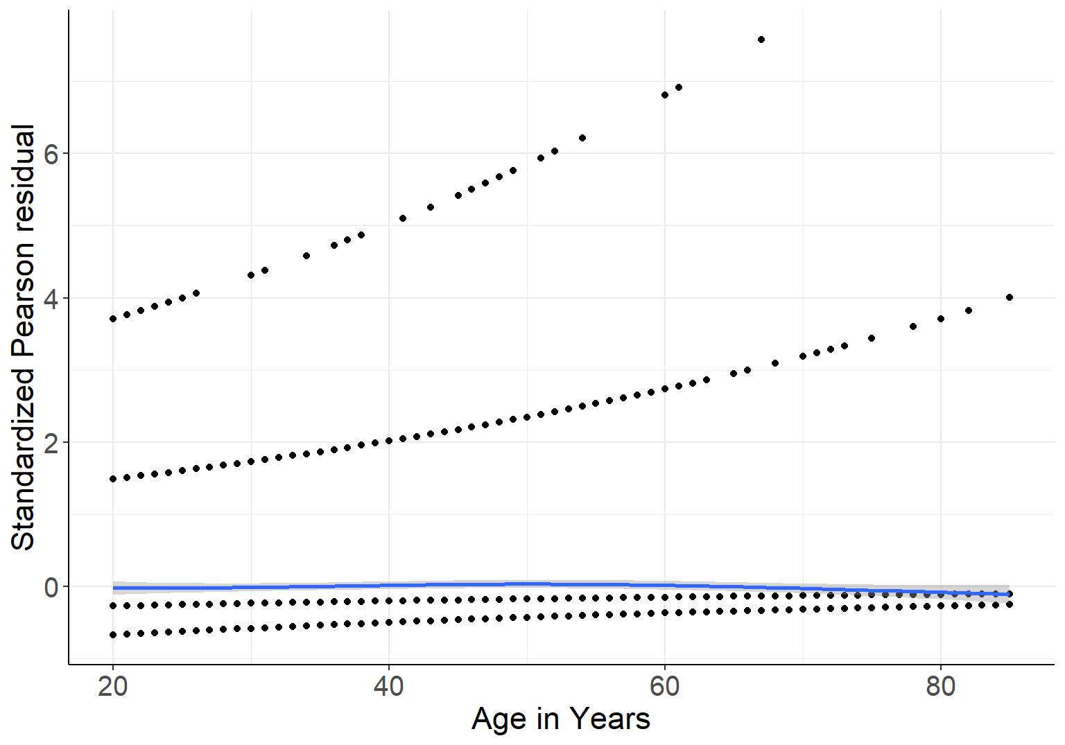
图 42.1: Standardized Pearson residuals agianst age, in logistic model with gender and linear age as covariates
图 42.1 中靠近横轴的蓝色实线是 LOWESS 平滑曲线,它十分接近平直的横线,也证明了 Pearson 标准化残差值和年龄本身并无关联。这同时也佐证了,将年龄以连续型共变量的形式放入本次逻辑回归模型中并非不合理 (not unreasonable)。
下一步,我们再来考虑,模型中加入 bmi 是否合理 (能改善模型的拟合度):
Model_NH3 <- glm(Heavydrinker ~ gender + ageyrs + bmi, data = NHANES, family = binomial(link = "logit"))
epiDisplay::logistic.display(Model_NH3) ; summary(Model_NH3)
Logistic regression predicting Heavydrinker

                    crude OR(95%CI)         adj. OR(95%CI)
gender (cont. var.) 0.17 (0.12,0.24)        0.16 (0.11,0.23)

ageyrs (cont. var.) 0.97 (0.97,0.98)        0.97 (0.96,0.98)

bmi (cont. var.)    0.9965 (0.9756,1.0179)  1.0084 (0.9855,1.0318)

                    P(Wald's test) P(LR-test)
gender (cont. var.) < 0.001        < 0.001

ageyrs (cont. var.) < 0.001        < 0.001

bmi (cont. var.)    0.477          0.479

Log-likelihood = -801.0412
No. of observations = 2548
AIC value = 1610.0825
Call:
glm(formula = Heavydrinker ~ gender + ageyrs + bmi, family = binomial(link = "logit"),
    data = NHANES)

Coefficients:
             Estimate Std. Error z value Pr(>|z|)
(Intercept)  1.425118   0.409603   3.479 0.000503 ***
gender      -1.829978   0.173818 -10.528  < 2e-16 ***
ageyrs      -0.030688   0.004011  -7.652 1.98e-14 ***
bmi          0.008346   0.011734   0.711 0.476905
---
Signif. codes:  0 '***' 0.001 '**' 0.01 '*' 0.05 '.' 0.1 ' ' 1

(Dispersion parameter for binomial family taken to be 1)

    Null deviance: 1810.2  on 2547  degrees of freedom
Residual deviance: 1602.1  on 2544  degrees of freedom
AIC: 1610.1

Number of Fisher Scoring iterations: 6
BMI的回归系数是否为零的Wald 检验\(p=0.477\),提示数据无法提供证据去反对零假设:“调整了年龄和性别之后,BMI 和是否是重度饮酒者的概率的对数比值\(\text{ log-odds}\) 之间无线性关系”,也就是二者之间可能有非线性关系。如果把 Pearson 标准化残差和 BMI 作残差散点图,如下所示:
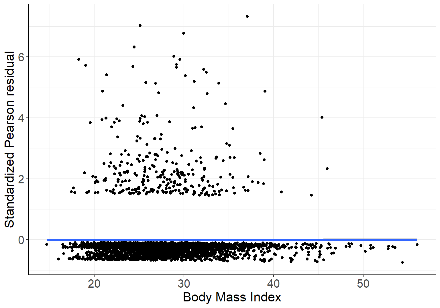
图 42.2: Standardized Pearson residuals agianst BMI, in logistic model with gender and linear age as covariates
此残差图 42.2 的 LOWESS 平滑曲线却提示我们,BMI 和残差之间不完全是毫无关系的 (应该是非线性的,抛物线关系?)。如果我们把 BMI 取平方放入模型中再看其结果:
NHANES <- mutate(NHANES, bmi2 = bmi^2)
Model_NH4 <- glm(Heavydrinker ~ gender + ageyrs + bmi + bmi2, data = NHANES, family = binomial(link = "logit"))
summary(Model_NH4)
Call:
glm(formula = Heavydrinker ~ gender + ageyrs + bmi + bmi2, family = binomial(link = "logit"),
    data = NHANES)

Coefficients:
             Estimate Std. Error z value Pr(>|z|)
(Intercept) -2.127753   1.480633  -1.437   0.1507
gender      -1.778443   0.174598 -10.186  < 2e-16 ***
ageyrs      -0.032379   0.004094  -7.910 2.58e-15 ***
bmi          0.255199   0.100329   2.544   0.0110 *
bmi2        -0.004123   0.001685  -2.446   0.0144 *
---
Signif. codes:  0 '***' 0.001 '**' 0.01 '*' 0.05 '.' 0.1 ' ' 1

(Dispersion parameter for binomial family taken to be 1)

    Null deviance: 1810.2  on 2547  degrees of freedom
Residual deviance: 1594.9  on 2543  degrees of freedom
AIC: 1604.9

Number of Fisher Scoring iterations: 6
Logistic regression predicting Heavydrinker

                    crude OR(95%CI)         adj. OR(95%CI)
gender (cont. var.) 0.17 (0.12,0.24)        0.17 (0.12,0.24)

ageyrs (cont. var.) 0.97 (0.97,0.98)        0.97 (0.96,0.98)

bmi (cont. var.)    1 (0.98,1.02)           1.29 (1.06,1.57)

bmi2 (cont. var.)   0.9999 (0.9995,1.0002)  0.9959 (0.9926,0.9992)

                    P(Wald's test) P(LR-test)
gender (cont. var.) < 0.001        < 0.001

ageyrs (cont. var.) < 0.001        < 0.001

bmi (cont. var.)    0.011          0.006

bmi2 (cont. var.)   0.014          0.007

Log-likelihood = -797.4554
No. of observations = 2548
AIC value = 1604.9108Likelihood ratio test
Model 1: Heavydrinker ~ gender + ageyrs
Model 2: Heavydrinker ~ gender + ageyrs + bmi + bmi2
#Df LogLik Df Chisq Pr(>Chisq)
1 3 -801.29
2 5 -797.46 2 7.6731 0.02157 *
---
Signif. codes: 0 '***' 0.001 '**' 0.01 '*' 0.05 '.' 0.1 ' ' 1通过似然比检验比较加了bmi, bmi2 两个共变量的模型和只有gender, ageyrs 两个共变量的模型\((p=0.022)\),提示我们BMI 和是否是重度饮酒者(概率的对数比值\(\text{log-odds}\)) 之间的关系并非简单的线性关系。不过这样的关系似乎并不是特别的明显,图 42.2 的平滑曲线的弯曲程度也没有特别明显。所以,在这样的情况下,有的统计学家可能还是会选择不放 BMI 进入模型里。
42.5 GLM例10
继续沿用 NHANES 数据,此次练习我们把重点放在收集到的收缩期血压数据上。定义收缩期血压大于 140 \(\text{mmHg}\) 者为高血压患者。
# 1. load the data and define a binary variable indicating whether
#    each observation has hypertension (1) or not (0)
NHANES <- haven::read_dta("../Datas/nhanesglm.dta")
NHANES <- NHANES %>%
  mutate(Gender = ifelse(gender == 1, "Male", "Female")) %>%
    mutate(Gender = factor(Gender, levels = c("Male", "Female")))
NHANES <- mutate(NHANES, hypertension = sbp >= 140)
tab1(NHANES$hypertension, graph = FALSE)
NHANES$hypertension :
Frequency Percent Cum. percent
FALSE 2116 83 83
TRUE 432 17 100
Total 2548 100 100# 2. Bearing in mind that we know blood pressure increases with age
# we begin by including age into a logistic regression for the
# the binary hypertension variable. We can use a lowess smoother
# plot to examine how the probability of hypertension varies with
# age.
pi <- with(NHANES, predict(loess(hypertension ~ ageyrs)))
with(NHANES, scatter.smooth(ageyrs, logit(pi), pch = 20, span = 0.6, lpars =
list(col = "blue", lwd = 3, lty = 1), col=rgb(0,0,0,0.004),
xlab = "Age in years",
ylab = "Logit(probability) of Hypertension",
frame = FALSE))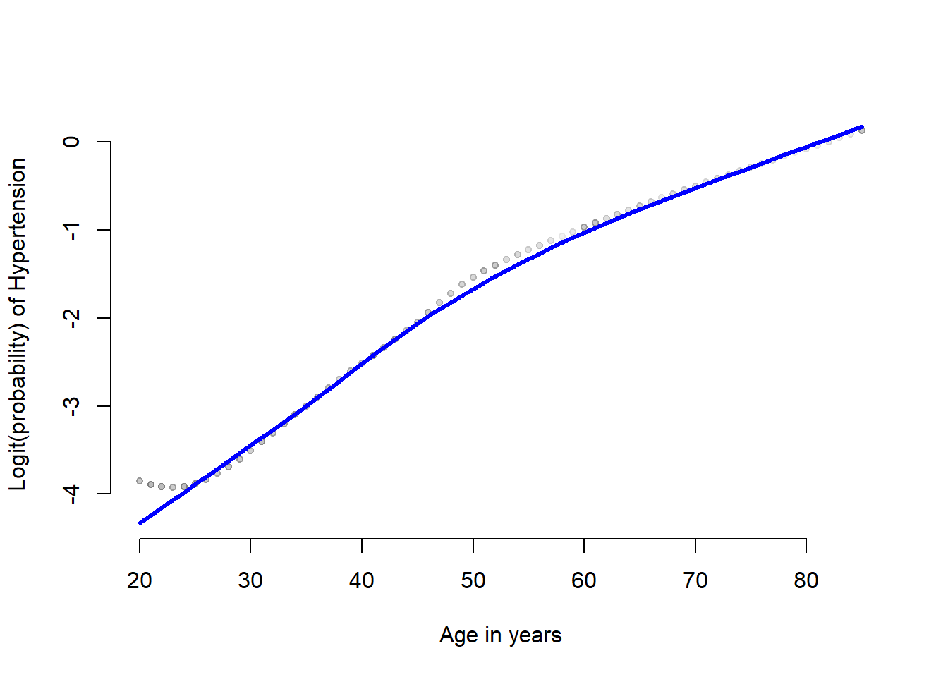
图 42.3: The loess plot of the observed proportin with hypertension against age. Span = 0.6
Lowess 平滑曲线图提示,高血压患病的可能性的 \(\text{logit}\),和年龄之间的关系似乎不是简单直线关系。我们可能需要把年龄本身和年龄的平方放入逻辑回归模型中去看看。
# 3. Include age into the logistic regression in the way suggested by the lowess plot.
#    do your results support your findings from the previous graph?
NHANES <- mutate(NHANES, agesq = ageyrs^2)
Model_NH5 <- glm(hypertension ~ ageyrs + agesq, data = NHANES, family = binomial(link = "logit"))
logistic.display(Model_NH5) ; summary(Model_NH5)
Logistic regression predicting hypertension

                    crude OR(95%CI)         adj. OR(95%CI)
ageyrs (cont. var.) 1.07 (1.06,1.07)        1.15 (1.1,1.21)

agesq (cont. var.)  1.0005 (1.0005,1.0006)  0.9993 (0.9989,0.9997)

                    P(Wald's test) P(LR-test)
ageyrs (cont. var.) < 0.001        < 0.001

agesq (cont. var.)  0.001          < 0.001

Log-likelihood = -943.7811
No. of observations = 2548
AIC value = 1893.5622
Call:
glm(formula = hypertension ~ ageyrs + agesq, family = binomial(link = "logit"),
    data = NHANES)

Coefficients:
              Estimate Std. Error z value Pr(>|z|)
(Intercept) -6.9293123  0.6720564 -10.311  < 2e-16 ***
ageyrs       0.1393366  0.0241990   5.758 8.51e-09 ***
agesq       -0.0006704  0.0002087  -3.212  0.00132 **
---
Signif. codes:  0 '***' 0.001 '**' 0.01 '*' 0.05 '.' 0.1 ' ' 1

(Dispersion parameter for binomial family taken to be 1)

    Null deviance: 2319.5  on 2547  degrees of freedom
Residual deviance: 1887.6  on 2545  degrees of freedom
AIC: 1893.6

Number of Fisher Scoring iterations: 6
正如同 Lowess 平滑曲线建议的那样,数据提供了极强的证据证明年龄和患有高血压概率的对数比值 \((\text{log-odds})\) 之间呈现的是抛物线关系。
# 4. Generate Pearson residuals and investigate whether the way in
#    which you have included age in the logistic regression in the
#    previous part is correct.

# obtain the standardized Pearson residuals by covariate pattern
Diag <- LogisticDx::dx(Model_NH5)
ggplot(Diag, aes(x = ageyrs, y = sPr)) +  geom_point() +
  geom_smooth(span = 0.9, se = FALSE) +  theme_bw()  +
  theme(axis.text = element_text(size = 15),
  axis.text.x = element_text(size = 15),
  axis.text.y = element_text(size = 15)) +
  labs(x = "Age in years", y = "standardised Pearson residual")  +
  theme(axis.title = element_text(size = 17), axis.text = element_text(size = 8),
        axis.line = element_line(colour = "black"),
    panel.border = element_blank(),
    panel.background = element_blank())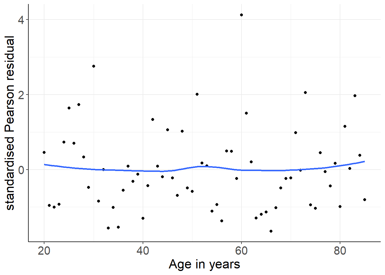
图 42.4: Standardized Pearson residuals (by covariate pattern) vs. age. Logistic mdoel with linear and quadratic age as covariates.
标准化 Pearson 残差 (共变量模式) 和年龄之间的散点图 42.4 提示此时的残差和年龄之间再无明显的关系。也就是说,年龄作为连续变量和高血压患病概率的对数比值之间的关系,用抛物线 (二次方程) 拟合并非不合理 (not unreasonable)。
# 5. Next, use individual level residuals to examine whether BMI ought to be
#    included in the model, and depending on what you find, continue with you
#    previous model or add BMI. In the latter case, generate new residuals and
#    assess if you have included BMI using the most appropriate functional form.
NHANES$stresPearson <- boot::glm.diag(Model_NH5)$rp
ggplot(NHANES, aes(x = bmi, y = stresPearson)) +
  geom_point() +
  theme_bw() +
  geom_smooth(span = 0.8, se = FALSE) +
  theme(axis.text = element_text(size = 15),
  axis.text.x = element_text(size = 15),
  axis.text.y = element_text(size = 15)) +
  labs(x = "Body Mass Index", y = "Standardized Pearson residual")  +
  theme(axis.title = element_text(size = 17), axis.text = element_text(size = 8),
        axis.line = element_line(colour = "black"),
    panel.border = element_blank(),
    panel.background = element_blank())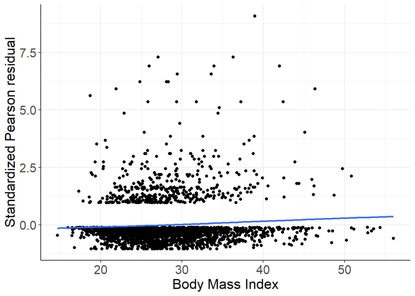
图 42.5: Standardized Pearson residuals vs. BMI. Logistic mdoel with just linear and quadratic age as covariates.
图 42.5,提示,标准化 Pearson 残差和连续型 BMI 值之间应该存在相关性,也就是该图提示需要加入连续型变量 BMI 进入逻辑回归模型中去!
Model_NH6 <- glm(hypertension ~ ageyrs + agesq + bmi, data = NHANES, family = binomial(link = "logit"))
logistic.display(Model_NH6) ; summary(Model_NH6)
Logistic regression predicting hypertension

                    crude OR(95%CI)         adj. OR(95%CI)
ageyrs (cont. var.) 1.07 (1.06,1.07)        1.14 (1.09,1.2)

agesq (cont. var.)  1.0005 (1.0005,1.0006)  0.9994 (0.999,0.9998)

bmi (cont. var.)    1.02 (1.01,1.04)        1.03 (1.01,1.05)

                    P(Wald's test) P(LR-test)
ageyrs (cont. var.) < 0.001        < 0.001

agesq (cont. var.)  0.005          0.004

bmi (cont. var.)    0.007          0.007

Log-likelihood = -940.1583
No. of observations = 2548
AIC value = 1888.3166
Call:
glm(formula = hypertension ~ ageyrs + agesq + bmi, family = binomial(link = "logit"),
    data = NHANES)

Coefficients:
              Estimate Std. Error z value Pr(>|z|)
(Intercept) -7.5411103  0.7101030 -10.620  < 2e-16 ***
ageyrs       0.1310800  0.0243081   5.392 6.95e-08 ***
agesq       -0.0005917  0.0002103  -2.814  0.00490 **
bmi          0.0284032  0.0104636   2.714  0.00664 **
---
Signif. codes:  0 '***' 0.001 '**' 0.01 '*' 0.05 '.' 0.1 ' ' 1

(Dispersion parameter for binomial family taken to be 1)

    Null deviance: 2319.5  on 2547  degrees of freedom
Residual deviance: 1880.3  on 2544  degrees of freedom
AIC: 1888.3

Number of Fisher Scoring iterations: 6
加入连续型变量 BMI 进入模型后,bmi 项的 Wald 检验结果果然证实了 之前残差图提示的 BMI 和高血压患病概率之间存在相关性。再对 Model_NH6 的残差和 bmi 作残差散点图:
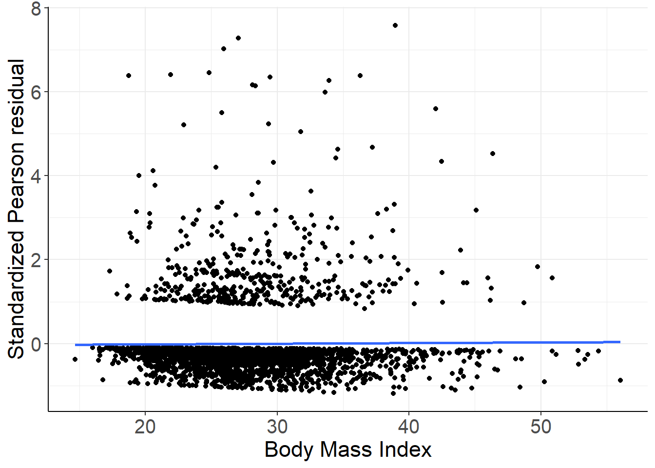
图 42.6: Standardized Pearson residuals vs. BMI. Logistic mdoel with linear and quadratic age and BMI as covariates.
现在的残差散点图提示残差和 bmi 之间不再有关系,所以之前把 bmi 加入逻辑回归模型是个并非不合理 (not unreasonable)的选择。
# 6. So far we have ingored gender. Explore whether gender should be included
#    in the model. including whether or not the other covariates included
#    already interact with gender with their effects on hypertension.
Model_NH7 <- glm(hypertension ~ ageyrs + agesq + bmi + Gender,
                 data = NHANES, family = binomial(link = "logit"))
logistic.display(Model_NH7) ; summary(Model_NH7)
Logistic regression predicting hypertension

                       crude OR(95%CI)         adj. OR(95%CI)
ageyrs (cont. var.)    1.07 (1.06,1.07)        1.14 (1.09,1.2)

agesq (cont. var.)     1.0005 (1.0005,1.0006)  0.9994 (0.999,0.9998)

bmi (cont. var.)       1.02 (1.01,1.04)        1.03 (1.01,1.05)

Gender: Female vs Male 1.1 (0.9,1.36)          1.24 (0.98,1.56)

                       P(Wald's test) P(LR-test)
ageyrs (cont. var.)    < 0.001        < 0.001

agesq (cont. var.)     0.005          0.004

bmi (cont. var.)       0.009          0.009

Gender: Female vs Male 0.07           0.07

Log-likelihood = -938.5164
No. of observations = 2548
AIC value = 1887.0328
Call:
glm(formula = hypertension ~ ageyrs + agesq + bmi + Gender, family = binomial(link = "logit"),
    data = NHANES)

Coefficients:
               Estimate Std. Error z value Pr(>|z|)
(Intercept)  -7.6441142  0.7140532 -10.705  < 2e-16 ***
ageyrs        0.1320636  0.0243597   5.421 5.91e-08 ***
agesq        -0.0005971  0.0002107  -2.834  0.00459 **
bmi           0.0273094  0.0104320   2.618  0.00885 **
GenderFemale  0.2121319  0.1170395   1.812  0.06991 .
---
Signif. codes:  0 '***' 0.001 '**' 0.01 '*' 0.05 '.' 0.1 ' ' 1

(Dispersion parameter for binomial family taken to be 1)

    Null deviance: 2319.5  on 2547  degrees of freedom
Residual deviance: 1877.0  on 2543  degrees of freedom
AIC: 1887

Number of Fisher Scoring iterations: 6Likelihood ratio test
Model 1: hypertension ~ ageyrs + agesq + bmi
Model 2: hypertension ~ ageyrs + agesq + bmi + Gender
#Df LogLik Df Chisq Pr(>Chisq)
1 4 -940.16
2 5 -938.52 1 3.2838 0.06997 .
---
Signif. codes: 0 '***' 0.001 '**' 0.01 '*' 0.05 '.' 0.1 ' ' 1# some evidence of an effect of gender.
# the Wald test and the likelihood ratio test are both borderline
# statistically significant.
Model_NH8 <- glm(hypertension ~ ageyrs + agesq + bmi*Gender,
data = NHANES, family = binomial(link = "logit"))
logistic.display(Model_NH8)
Logistic regression predicting hypertension

                       crude OR(95%CI)         adj. OR(95%CI)
ageyrs (cont. var.)    1.07 (1.06,1.07)        1.14 (1.09,1.2)

agesq (cont. var.)     1.0005 (1.0005,1.0006)  0.9994 (0.999,0.9998)

bmi (cont. var.)       1.02 (1.01,1.04)        1.05 (1.01,1.08)

Gender: Female vs Male 1.1 (0.9,1.36)          3.01 (0.9,10)

bmi:GenderFemale       -                       0.97 (0.93,1.01)

                       P(Wald's test) P(LR-test)
ageyrs (cont. var.)    < 0.001        < 0.001

agesq (cont. var.)     0.006          0.005

bmi (cont. var.)       0.005          1

Gender: Female vs Male 0.072          0.072

bmi:GenderFemale       0.139          0.139

Log-likelihood = -937.423
No. of observations = 2548
AIC value = 1886.846Likelihood ratio test
Model 1: hypertension ~ ageyrs + agesq + bmi + Gender
Model 2: hypertension ~ ageyrs + agesq + bmi * Gender
#Df LogLik Df Chisq Pr(>Chisq)
1 5 -938.52
2 6 -937.42 1 2.1867 0.1392# no strong evidence of an interaction between BMI and gender
# from both wald test and likelihood ratio test.
Model_NH9 <- glm(hypertension ~ ageyrs*Gender + agesq + bmi,
data = NHANES, family = binomial(link = "logit"))
logistic.display(Model_NH9)
Logistic regression predicting hypertension

                       crude OR(95%CI)         adj. OR(95%CI)
ageyrs (cont. var.)    1.07 (1.06,1.07)        1.13 (1.08,1.19)

Gender: Female vs Male 1.1 (0.9,1.36)          0.34 (0.14,0.84)

agesq (cont. var.)     1.0005 (1.0005,1.0006)  0.9994 (0.999,0.9998)

bmi (cont. var.)       1.02 (1.01,1.04)        1.03 (1.01,1.05)

ageyrs:GenderFemale    -                       1.02 (1.01,1.04)

                       P(Wald's test) P(LR-test)
ageyrs (cont. var.)    < 0.001        1

Gender: Female vs Male 0.02           0.018

agesq (cont. var.)     0.004          0.003

bmi (cont. var.)       0.008          0.009

ageyrs:GenderFemale    0.004          0.004

Log-likelihood = -934.2658
No. of observations = 2548
AIC value = 1880.5315Likelihood ratio test
Model 1: hypertension ~ ageyrs + agesq + bmi + Gender
Model 2: hypertension ~ ageyrs * Gender + agesq + bmi
#Df LogLik Df Chisq Pr(>Chisq)
1 5 -938.52
2 6 -934.27 1 8.5013 0.003549 **
---
Signif. codes: 0 '***' 0.001 '**' 0.01 '*' 0.05 '.' 0.1 ' ' 1Likelihood ratio test
Model 1: hypertension ~ ageyrs + agesq + bmi
Model 2: hypertension ~ ageyrs * Gender + agesq + bmi
#Df LogLik Df Chisq Pr(>Chisq)
1 4 -940.16
2 6 -934.27 2 11.785 0.00276 **
---
Signif. codes: 0 '***' 0.001 '**' 0.01 '*' 0.05 '.' 0.1 ' ' 1增加性别项进入逻辑回归模型以后,数据提供了临界有意义证据 \((p = 0.070)\) 证明了调整了年龄和 BMI 以后,高血压的患病概率依然和性别有关系。增加了 BMI 和性别的交互作用项之后发现,无证据证明性别和 BMI 之间存在有意义的交互作用 \((p=0.139)\)。但是,增加了年龄和性别的交互作用项以后,发现了有很强的证据证明性别和年龄之间存在交互作用 \((p=0.004)\)。增加性别以及性别和年龄的交互作用项,显著提升了模型对数据的拟合度 \((p = 0.0028)\)。此处,我们可以下结论认为,虽然加入年龄本身,对模型拟合程度提升有有限的帮助,但是当模型考虑了年龄和性别的交互作用之后,拟合数据的程度得到极为显著的改善。
当然,想要继续下去也是可以的,例如Model_NH9 的前提下,再加入年龄平方与性别的交互作用项,会发现其Wald 检验结果提示年龄平方,和性别的交互作用是没有意义的\(( p=0.58)\)。
# 7. Based on your final model, calculate fitted probabilities for an individual
#    aged 60 years, at BMI values from 20 to 40 in increments of 5, separately
#    for men and women, and plot the resulting values.

a <- data.frame(bmi = seq(20, 40, 5), ageyrs = rep(60, 5), agesq = rep(3600, 5), Gender = factor(rep("Male", 5)))
b <- data.frame(bmi = seq(20, 40, 5), ageyrs = rep(60, 5), agesq = rep(3600, 5), Gender = factor(rep("Female", 5)))

Predict_men <- predict(Model_NH9, a, se.fit = TRUE)$fit
Predict_men_se <- predict(Model_NH9, a, se.fit = TRUE)$se.fit
Point_pred_men <- exp(Predict_men)/(1+exp(Predict_men))
PredictCI_men_L <- exp(Predict_men - 1.96*Predict_men_se)/(1+exp(Predict_men- 1.96*Predict_men_se))
PredictCI_men_U <- exp(Predict_men + 1.96*Predict_men_se)/(1+exp(Predict_men+ 1.96*Predict_men_se))
cbind(Point_pred_men, PredictCI_men_L, PredictCI_men_U)
Point_pred_men PredictCI_men_L PredictCI_men_U
1 0.2099999 0.1699024 0.2566349
2 0.2340988 0.1998047 0.2722762
3 0.2600528 0.2257591 0.2975539
4 0.2878031 0.2441125 0.3358391
5 0.3172450 0.2570154 0.3842887Predict_women <- predict(Model_NH9, b, se.fit = TRUE)$fit
Predict_women_se <- predict(Model_NH9, b, se.fit = TRUE)$se.fit
Point_pred_women <- exp(Predict_women)/(1+exp(Predict_women))
PredictCI_women_L <- exp(Predict_women - 1.96*Predict_women_se)/(1+exp(Predict_women- 1.96*Predict_women_se))
PredictCI_women_U <- exp(Predict_women + 1.96*Predict_women_se)/(1+exp(Predict_women+ 1.96*Predict_women_se))
cbind(Point_pred_women, PredictCI_women_L, PredictCI_women_U) Point_pred_women PredictCI_women_L PredictCI_women_U
1 0.2491342 0.2007652 0.3047135
2 0.2761542 0.2347806 0.3217531
3 0.3049146 0.2647727 0.3482597
4 0.3352829 0.2865948 0.3877467
5 0.3670785 0.3019196 0.4374868