第 22 章前提和数据转换

几乎所有的统计分析手法都有自己的前提条件，所以重要的问题来了：

在多大的程度上分析结果引导的结论会依赖于这些前提？
有没有方法检验，至少检查数据是否满足前提条件？
如果数据无法满足相应的前提条件，该怎么办？

目前为止，分析方法中接触到的简单统计检验法中典型的前提举例如下：

单样本 \(t\) 检验 (Section 19.3.3) 需要的前提条件是所有的观察数据
- 相互独立 independent；
- 服从正态分布 normally distributed。
事件发生率的置信区间计算 (Section 18.8) 需要的前提条件是
- 事件发生的件数服从泊松分布 Poisson distributed。
两个百分比的卡方检验 (Section 20.3.3 and Section 21.3.1) 需要的前提条件是
- 两组数据中成功次数的数据服从二项分布 Binomial distributed。

当观察数据可能不满足上述前提条件时，一个最为常用的手段是对原始数据进行数学转换 (transformation)。然而，数学转换会对推断的结果意义产生影响：

数学转换以后的数据可能更加满足前提条件，不好的数学转换则可能使转换后的数据更加偏离前提条件；
数学转换以后，改变了统计结果的现实意义，change the ease of interpretation of the results。

比方说，一组采样获得的血压数据，你发现把原始数据开根号之后的结果可以符合正态分布的前提，但是此种转换最大的缺点是，转换后的数据使用two sample \(t\) test时比较的不再是均值差，而是开根号之后的差。这就导致了无法良好的解释这样的差异在实际生活中有什么意义(临床上的意义)，换句话说，医生和患者是无法理解什么是根号血压差的\(\sqrt{ \text{mmHg}}\)。

22.1 稳健性

其实应用统计学方法时真实数据多多少少会偏离一些前提条件，在某些前提条件不能满足的情况下，分析结果是否稳健 (robustness) 有如下不太精确但是广泛被接受的定义：

那么什么情况下可以说一个统计方法是表现良好的呢，performing well？

我们说一个统计方法表现良好，是指该方法用于定义是否有意义的临界值，或者叫名义显著性水平(nominal signficance level)，和实际上计算的检验统计量在所有的可能中达到或超过该临界值的概率(actual probability the test statistic exceeds the cut-off)。用 \(t\) 检验举例如下：

\[ \text{Prob}(|T| > t_{df,0.975} | \text{H}_0 \text{true}) = 0.05 \]

类似地，我们说一个置信区间的计算方法表现良好，是指该方法计算获得的 \(95\%\) 置信区间包含真实参数值的概率真的可以无限接近 \(95\%\)：

\[ \text{Prob}(\mu \in (L, U) | \mu) = 0.95 \]

一些常见方法的稳健性列举：

样本量小且分布偏度越大时，依赖正态分布前提的置信区间计算和其他的检验手段就变得不再可靠；
两个方差比较时使用的 \(F\) 检验 (Section 21.2.1 ) 常常由于数据不服从正态分布缺乏稳健性，即使样本量较大也不能改善；
根据中心极限定理，样本量足够大时，单样本 \(t\) 检验 (Section 19.3.3 ) 具有良好的稳健性。
一般地，基于均值的检验方法都相对其他统计量较为稳健。

22.2 正态性

大多数情况下，正如我们在这个部分最开头的章节提到的，拿到数据以后先用图形手段探索，并熟悉该数据。从图形来判断一组数据是否接近正态分布或者偏离正态分布。常用的探索连续型变量是否服从正态分布的图形方法是：

箱形图，box and whisker plot，如图 17.5；
柱状图，histogram，如图 22.1；
正态分布图，normal plots，如图 22.2。

set.seed(99)
Normal <- rnorm(2500, mean = 120, sd = 8)
h <- hist(Normal,breaks = 20, col = "lightblue", xlab = "some value" ,
          ylim = c(0,300))
xfit<-seq(min(Normal),max(Normal),length=40)
yfit<-dnorm(xfit,mean=mean(Normal),sd=sd(Normal))
yfit <- yfit*diff(h$mids[1:2])*length(Normal)
lines(xfit, yfit, col="blue", lwd=2)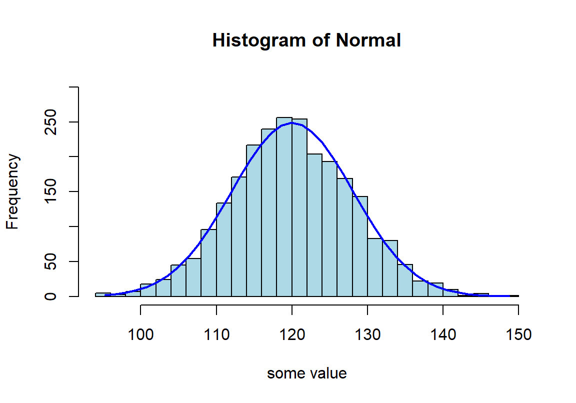

图 22.1: Appearance of histogram with normal curve

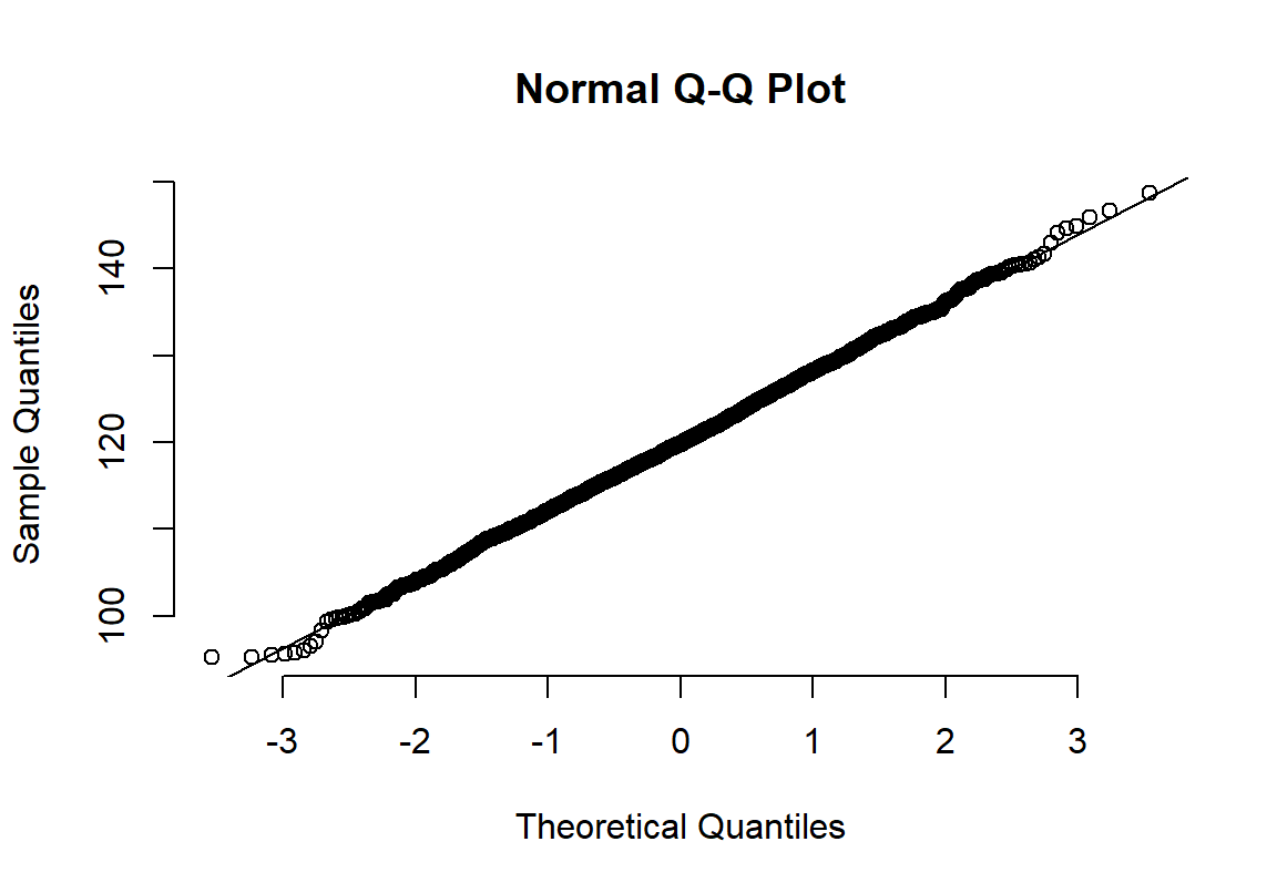
qqnorm(Normal,frame=F); qqline(Normal)

图 22.2: Appearance of normal plot for a normally distributed variable

22.2.1 正态分布图 normal plot

其实光看柱状图和箱形图，有时候很难判断数据正态性与否，当数据和正态分布有些微妙的不同时可能就没办法从柱状图觉察出来。此时需要借用正态分布图的威力。正态分布图的原理就是，把原始数据 (Y轴) 和理论上服从正态分布的期待数据 (X轴) 从小到大排序一一对应以后绘制散点图。所以理论上，如果原始数据服从正态分布，那么正态分布中第10百分位的点，我们期望和原始数据中第10百分位的点十分接近，那么绘成的散点图应该接近于完美的贴在\(y=x\) 这条直线上。如果正态分布图的点越偏离 \(y=x\) 的直线，觉说明原始数据越偏离正态分布。

下面的系列图22.3，22.4，22.5，@ref(fig:skewneg -hist-normal)展示了各种非正态分布时会出现的柱状图，和正态分布图的特征：

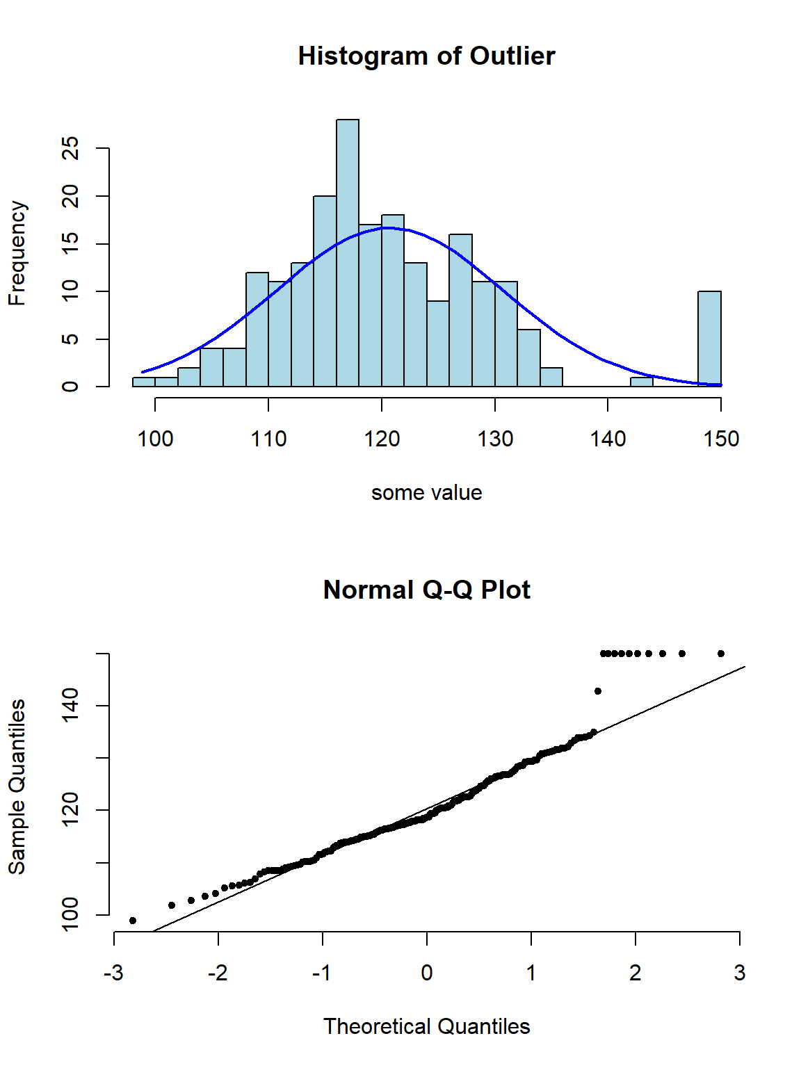
图 22.3: Appearance of histogram and normal plot for a variable with outlying values

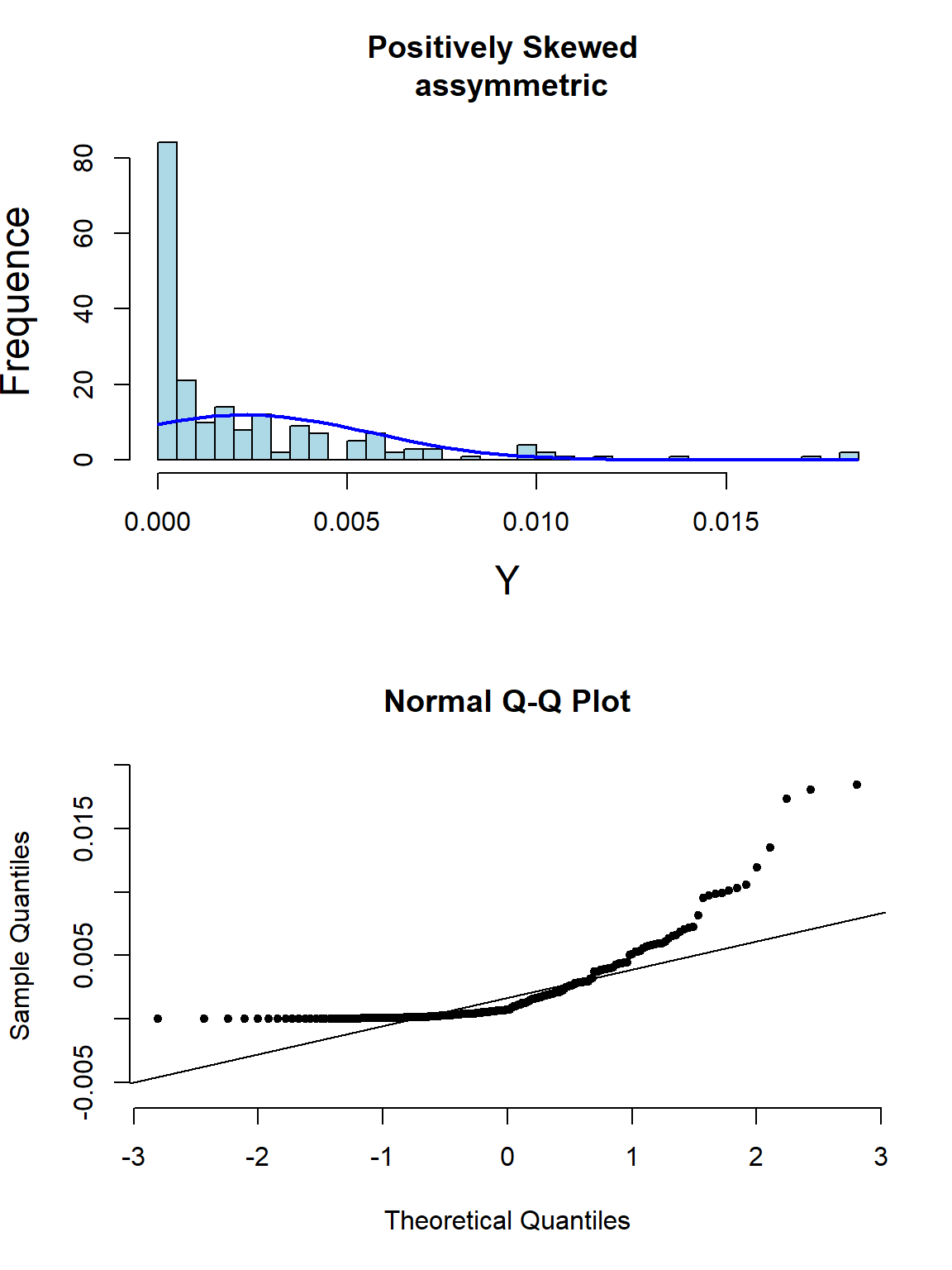
图 22.4: Appearance of histogram and normal plot for a variable exhibiting right-skewness

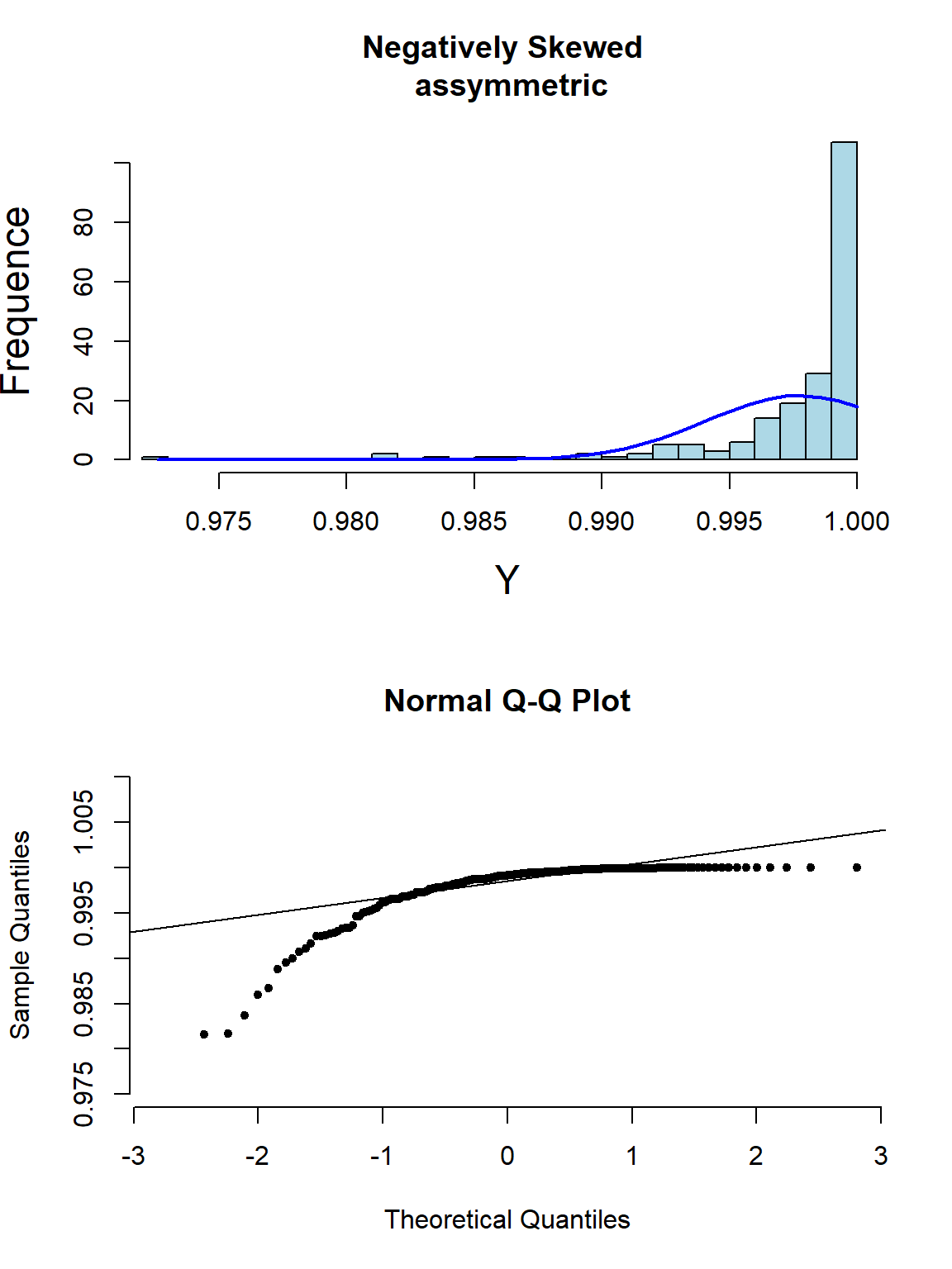
图 22.5: Appearance of histogram and normal plot for a variable exhibiting left-skewness

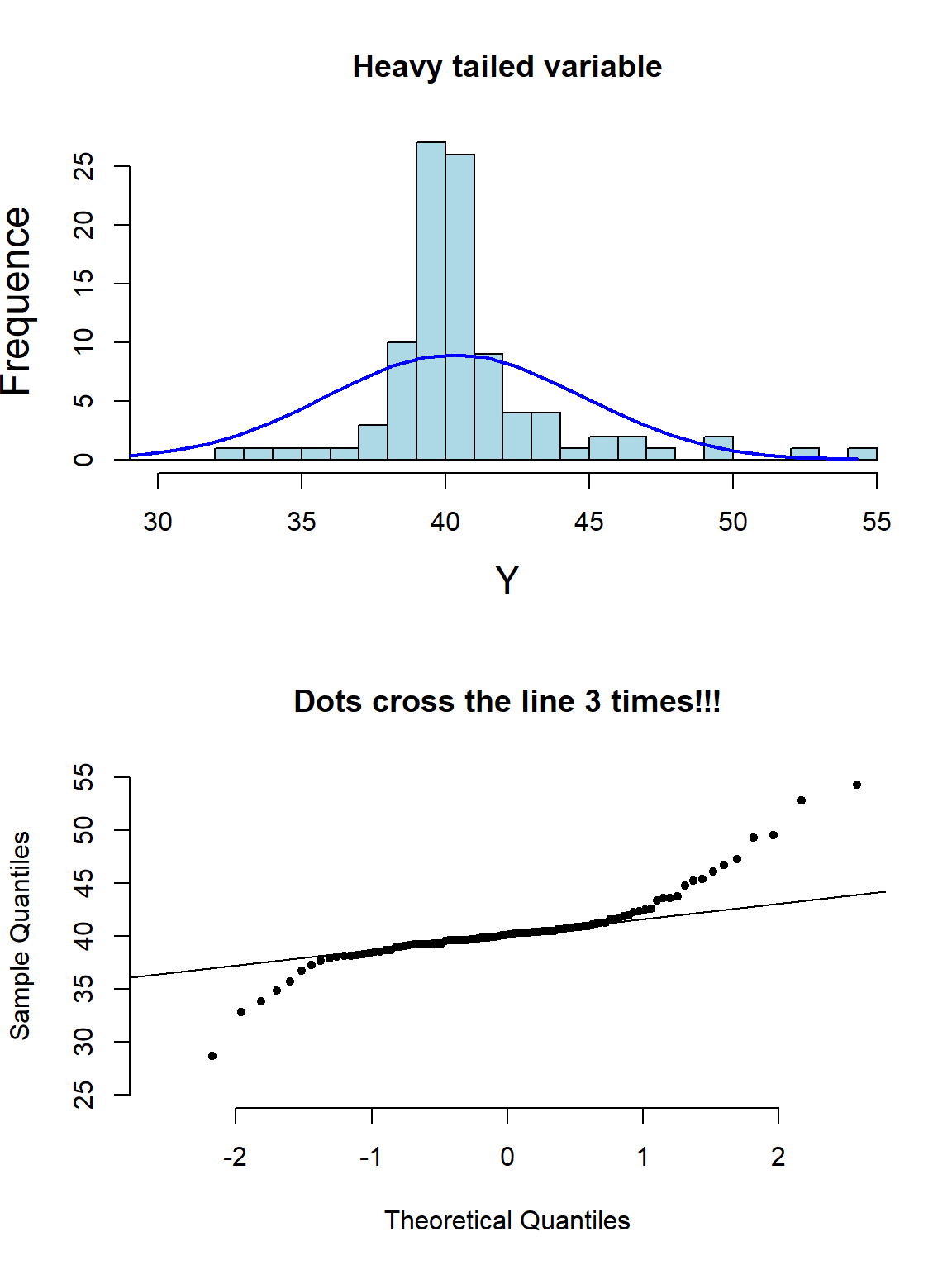
图 22.6: Appearance of histogram and normal plot for a heavy tailed variable

如果对数据是否服从正态分布实在没有信心，统计学家也很少使用那些检验是否服从正态分布的所谓检验方法(Sharpiro-Wilk test 或者Kolmogorov-Smirnov test)，而是倾向用直接改用稳健统计学分析法(Robust Statistical Methods)。

22.3 总结连续型变量不服从正态分布时的处理方案

根据中心极限定理，样本量足够大时，即使原始样本数据不服从正态分布，仍然可以用一般的参数估计技巧来分析类似均值这样较为稳健的参数。
用非参数检验法，会在稳健统计学方法中介绍，但是这些方法的缺点很明显，例如无法进行精确的参数估计，且容易失去较大的统计学检验力(loss of power)，增加一类错误概率(错误的拒绝掉可能存在有意义差异的检验)。更重要的是，没有一种非参数检验法是可以和多重线性回归等较为复杂，高级的技巧等价的。
用一些稳健统计学方法 (bootstrap，“sandwich” estimators of variance)，可行但是对电脑的计算需求较高。
数据转换法。但是没有人能保证一定能找到合适的数学转换法来满足前提条件 (下节讨论)。

22.4 数学幂转换

数据转换家族：

\[ \cdots,x^{-2},x^{-1},x^{-\frac{1}{2}},\text{log}(x),x^{\frac{1}{2 }},x^1,x^2,\cdots \]

上面举例的数学幂转换方法，都是常见的手段用于降低原始数据的偏度 (skewness)，相反地，幂转换却不一定能够改变数据的峰度 (kurtosis)。下面的方程，(非常的罗嗦的方程sorry)，用于实施类似ladder 在Stata 中的效果，即对数据进行各种转换，然后输出每种幂转换后的数据是否为正态分布的检验结果(使用shapiro.test())：

Ladder.x <- function(x){
    data <- data.frame(x^3,x^2,x,sqrt(x),log(x),1/sqrt(x),1/x,1/(x^2),1/(x^3))
    names(data) <- c("cubic","square","identity","square root","log","1/(square root)",
                     "inverse","1/square","1/cubic")
   # options(scipen=5)
    test1 <- shapiro.test(data$cubic)
    test2 <- shapiro.test(data$square)
    test3 <- shapiro.test(data$identity)
    test4 <- shapiro.test(data$`square root`)
    test5 <- shapiro.test(data$log)
    test6 <- shapiro.test(data$`1/(square root)`)
    test7 <- shapiro.test(data$inverse)
    test8 <- shapiro.test(data$`1/square`)
    test9 <- shapiro.test(data$`1/cubic`)
    W.statistic <- c(test1$statistic,
                     test2$statistic,
                     test3$statistic,
                     test4$statistic,
                     test5$statistic,
                     test6$statistic,
                     test7$statistic,
                     test8$statistic,
                     test9$statistic)
    p.value <- c(test1$p.value,
                 test2$p.value,
                 test3$p.value,
                 test4$p.value,
                 test5$p.value,
                 test6$p.value,
                 test7$p.value,
                 test8$p.value,
                 test9$p.value)
    Hmisc::format.pval(p.value ,digits=5, eps = 0.00001, scientific = FALSE)
    Transformation <- c("cubic","square","identity","square root","log","1/(square root)",
                        "inverse","1/square","1/cubic")
    Formula <- c("x^3","x^2","x","sqrt(x)","log(x)","1/sqrt(x)","1/x","1/(x^2)","1/(x^3)")
    (results <- data.frame(Transformation, Formula, W.statistic, p.value))
  }

Normal <- rnorm(2500, mean = 120, sd = 8)
Ladder.x(Normal)

##    Transformation   Formula W.statistic      p.value
## 1           cubic       x^3   0.9900758 3.905882e-12
## 2          square       x^2   0.9968146 4.283393e-05
## 3        identity         x   0.9993658 5.834687e-01
## 4     square root   sqrt(x)   0.9990492 2.039226e-01
## 5             log    log(x)   0.9976667 8.749798e-04
## 6 1/(square root) 1/sqrt(x)   0.9952199 3.369682e-07
## 7         inverse       1/x   0.9917142 8.895741e-11
## 8        1/square   1/(x^2)   0.9815677 1.734734e-17
## 9         1/cubic   1/(x^3)   0.9673507 2.175083e-23

22.4.1 对数转换

在众多幂转换中，对数转换是最常用的，因为对数转换之后，再通过逆运算转换回原单位数据的方法，被发现是相较于其他幂转换较为容易解释和应用在临床医学中。假如现在在分析男女之间收缩期血压的均值差别。下面是对数转换前后的检验方法步骤，试作一个对比：

转换前：

计算收缩期血压在男性女性中各自的均值 \(\bar{Y}_j, j=1,2\)；
计算男女间均值差 \(D=\bar{Y}_2 - \bar{Y}_1\)；
所以均值差就被解释为男女减血压的平均差距 (difference of mmHg)；
例如，均值差为 10 mmHg，就可以被解读为女性血压平均值比男性低 10 mmHg。

对数转换后：

计算观察值的对数值 \(t_{ij} = \text{log}_e(y_{ij})\)；
计算男女对数收缩期血压的算数平均值 \(\bar{T}_j, j=1,2\)；
计算对数血压均值差 \(D=\bar{T}_2-\bar{T}_1\)；
由于\(exp(\bar{T}_j) = G_j\) 是男女收缩期血压的几何平均值，所以\(exp(D)=exp(\text{log}_eG_2 - \text{log}_eG_1) = \ frac{G_2}{G_1}\)，就可以解释为男女收缩期血压的几何平均值之比；
例如，\(D=-0.05\)，那么男女收缩期血压的几何平均值之比为 \(exp(-0.05)=0.951\)，就可以被解读为女性收缩期血压平均比男性低 \(4.9\%\)。

22.4.2 逆转换置信区间

当使用转换后数据计算置信区间以后，需要再把数据逆转换回原始数据的单位才能顺利被解读。但是逆转换回去以后的置信区间就不再左右对称了 (no way)。

22.4.3 对数正态分布

一个随机变量的对数转换如果服从正态分布，我们说这个数据服从对数正态分布。

22.4.4 百分比的转换

百分比被局限在 \([0,1]\) 的范围内，所以为了打破这个取值范围的限制，百分比常用的数学转换有：

把百分比 \(\pi\) 转换成 Odds \(\frac{\pi}{1-\pi}\)。如此 Odds 的取值范围就可以变成 \([0, \infty)\)；
Odds \(\frac{\pi}{1-\pi}\) 又常被转换成 log-odds \(\text{log}(\frac{\pi}{1-\pi})\)。这样的转换方程 \(f(\pi)=\text{log}(\frac{\pi}{1-\pi})\) 又被命名为逻辑转换 (logit transformation)；
百分比的商 (危险度比，risk ratio) \(\pi_1/\pi_2\) 可以转换成 \(\text{log}(\pi_1/\pi_2)\)；
比值比(odds ratio) \(\frac{\pi_1(1-\pi_2)}{\pi_2(1-\pi_1)}\) 可以转换成对数比值比(log odds ratio) \(\text{log}[ \frac{\pi_1(1-\pi_2)}{\pi_2(1-\pi_1)}] = \text{log}[\pi_1(1-\pi_1)] - \text{log}[\pi_2(1 -\pi_2)]\)。

Common Transformation and their range
Transformation	Formula	Range
Odds	\(\frac{\pi}{1-\pi}\)	\([0,\infty)\)
Log Odds	\(\text{log}(\frac{\pi}{1-\pi})\)	\((-\infty,+\infty)\)
Risk Ratio	\(\frac{\pi_1}{\pi_2}\)	\([0,\infty)\)
Log Risk Ratio	\(\text{log}(\frac{\pi_1}{\pi_2})\)	\((-\infty,+\infty)\)
Odds Ratio	\(\frac{\pi_1(1-\pi_2)}{\pi_2(1-\pi_1)}\)	\([0,\infty)\)
Log Odds Ratio	\(\text{log}[\frac{\pi_1(1-\pi_2)}{\pi_2(1-\pi_1)}]\)	\((-\infty,+\infty)\)

第 22 章 前提和数据转换