第 50 章 纵向研究数据
本章我们来把目前为止了解的混合效应 (截距/斜率) 模型应用到一种特殊形态的数据 – 纵向研究数据 – 中去。
纵向数据,是一种前瞻性收集的来的数据,它随着时间的推移,在不同的时间点对相同的观察对象进行数据的采集。每个研究对象被收集数据时的时间点,可以是相同的,也可以是不同的。在很多临床实验中,患者被观察随访,并且常常在同样的时间点收集数据,所以在临床实验的特殊形态下,每个患者收集数据的时间点可以做到统一,这样的纵向研究数据是属于固定测量时刻的类型(fixed occasions)。但是在流行病学等观察性研究中获得的数据,就没有这么幸运,他们通常测量收集数据的时间点就不太可能保持一致,收集时间点不一致的纵向数据属于不固定测量时刻的类型(variable occasions)。
纵向数据英文名是longitudinal data,它的常见别的名称是重复测量数据(repeated measures data),计量经济学中叫做面板型数据(panel data),或者是时间序列横断面研究数据(cross sectional time series data)。所以在纵向数据这种特殊形态的的嵌套式数据结构中,第二层级结构就是一个个的个体,第一层级结构,就是每个个体在不同的时间点获得的测量值。除了和前面几章讨论过的嵌套式数据结构相似可以应用混合效应模型,纵向数据还有一些自己独特的性质需要加以考量:
- 层内数据的相关性结构是有测量时间的先后顺序的;
- 之前讨论的嵌套式结构数据在层内的观察值则没有严格的时间或者大小的排序 (例如同一所学校的不同学生);
- 换句话说,层内相关系数 (intra-class correlation) 很难被认为是相似或者相同的。
50.1 缺失值 Missing data
当纵向数据中存在一些缺失值,即使你在计算一些简单的归纳性分析,也要特别特别特别地小心。如果不是所有人都有全部测量时间点的数据的话,总体的平均特征数据分析了也没有太大的卵用,因为缺失值导致这样计算获得的并不是真实的平均值(也因为不同的患者,贡献了不同时间点的数据,没办法平均)。
如果存在缺失值,那么当且仅当这些缺失值和观测值 \(Y\) 之间没有关系时,才能认为这些简单计算和简单模型的建立是不带有偏倚的。如果说,有些缺失值确实是根据观测数据有选择性地缺失 (the mechanism driving the selection depends on measured data),随机效应模型的建立可以自动化校正这样的缺失,从而保证估计无偏。
根据观测数据选择性地出现缺失值的机制被叫做随机缺失 (Missing at random, MAR)。
50.2 固定测量时刻 fixed occasions
对于临床试验中固定时刻随访收集到的病人数据,理想状态下应该是一种平衡数据 (balanced data)。也就是在不同时间\(t_i , i = 1, \cdots, n\) 我们成功收集到所有患者的所有数据,所以每层(名患者) 拥有的时间序列数据的样本量是相同的\(n_j = n, \forall j\)。
如同分析其他类型的数据一样,分析纵向数据也要从描述数据开始。如果是平衡数据,描述性分析就很容易,当有缺失值时,分析就变得有些棘手。例如,我们可以计算每个时间点的平均值作为所有患者的 “平均特质 average profiles”。或者也可以用每个人的时间序列数据对时间做简单线性回归模型,从而获取每个个体的截距和斜率。
50.2.1 随机截距模型 random intercept model
复合对称模型 compound symmetry model, 是常见的一种用于重复测量数据的模型,它是基于随机截距模型的一种扩展模型。
当模型中没有解释变量时,
\[ \begin{equation} Y_{ij} = \mu_i + u_{0j} + e_{ij} \end{equation} \tag{50.1} \]
其中,
- \(i\) 是测量时刻;
- \(j\) 是实验的个体;
- \(\mu_i\) 是测量时刻 \(i\) 时的平均截距 – 这是一个固定效应。
为了拟合这个模型,我们需要先生成一系列的哑变量用来表示不同的测量时刻:
\[ Y_{ij} = \sum_{h=1}^n\beta_{0h} I_{i = h,j} + u_{0j} + e_{ij} \]
其中,
- \(I_{i = h,j}\) 是用于表示第 \(j\) 名患者的 \(i\) 次观测值,在第 \(h\) 次测量时是否被测量到的哑变量。
- 该模型暗示同一个患者收集到的不同时刻的观察数据是可以互换的,有相同的协方差 \[ \begin{aligned} \text{Cov}(Y_{1j} , Y_{2j}) & = \text{Cov}(u_{0j} + e_{1j}, u_{0j} + e_{2j}) \\ & = \sigma^2_{u_{00}} \end{aligned} \]
- 该模型还有另一个暗示是,不同患者之间任意时间点的两个观察数据之间是相互独立的 \[ \begin{aligned} \text{Cov}(Y_{1j}, Y_{2j*}) & = \text{Cov}(u_{0j} + e_{1j}, u_{0j*} + e_{2j*}) \\ & = 0 \end{aligned} \]
所以当没有缺失值时,数据是固定测量时刻(fixed occation) 的数据也是是平衡数据,那么每一个患者(第二层级数据) 的观察值可以写作是一个向量\(\{ \mathbf{Y}_ {ij} \}\),每名患者的观察值向量的长度都是相同的\(n\)。所以,它们的 \(n\times n\) 协方差矩阵就是:
\[ \Omega_y = \left( \begin{array}{cccc} \sigma^2_{u_{00}} + \sigma^2_e & \sigma^2_{u_{00}} & \cdots & \sigma^2_{u_{00}} \\ \sigma_{u_{00}} & \sigma^2_{u_{00}} + \sigma^2_e & \cdots & \sigma^2_{u_{00}} \\ \vdots & \vdots & \vdots & \vdots \\ \sigma^2_{u_{00}} & \sigma^2_{u_{00}} & \cdots & \sigma^2_{u_{00}} + \sigma^2_e\\ \end{array} \right) \]
也正是由于观测值的协方差矩阵是如此地对称,该模型被命名为复合对称模型 compound symmetric model。
- Adult height measures 数据
有(闲人)花了数十年时间追踪随访了近2000名女性在 26 岁,36岁,43岁,53岁时的身高。忽略掉可能存在的测量误差,研究者想知道是否随着年龄增加,女性的身高会缩水。这些女性在这些年龄时的身高数据总结如下:
##
## No. of observations = 2187
##
##   Var. name obs. mean   median  s.d.   min.   max.
## 1 ht26      1758 162.33 162.6   6.36   142.2  180.3
## 2 ht36      1610 162.26 162.2   6.05   135.2  180
## 3 ht43      1567 162.28 162.1   5.96   140    180
## 4 ht53      1462 161.56 161.5   5.96   134.3  179.6
原则上每个女性在所有的时间应该都有身高测量值才对,我们暂且认为拥有缺失测量值的时间点是完全随机的。先计算样本中数据完整部分的女性身高在四个时间点时的方差协方差矩阵:
##          ht26     ht36     ht43     ht53
## ht26 39.81340 34.75846 34.47898 34.12817
## ht36 34.75846 34.45506 33.36041 33.08668
## ht43 34.47898 33.36041 34.33150 32.94885
## ht53 34.12817 33.08668 32.94885 34.21519
要给这个数据拟合混合对称模型(compound symmetry model),需要先把数据从宽变长,之后为每个测量身高的时间点生成一个哑变量,然后拟合无截距式的随机截距模型:
# 把数据格式从宽变长
hei_long <- height %>%
  gather(key, value, -id, -bw, -mht) %>%
    separate(key, into = c("Height", "H_Age"), sep = 2) %>%
      arrange(id, H_Age, bw, mht) %>%
        spread(Height, value)

# 生成四个年龄时间点数据的哑变量
hei_long <- hei_long %>%
  mutate(Age_1 = ifelse(H_Age == 26, 1, 0),
         Age_2 = ifelse(H_Age == 36, 1, 0),
         Age_3 = ifelse(H_Age == 43, 1, 0),
         Age_4 = ifelse(H_Age == 53, 1, 0))
M_hei <- lmer(ht ~ 0 + Age_1 + Age_2 + Age_3 + Age_4 + (1 | id), data = hei_long, REML = TRUE)
summary(M_hei)
## Linear mixed model fit by REML. t-tests use Satterthwaite's method [
## lmerModLmerTest]
## Formula: ht ~ 0 + Age_1 + Age_2 + Age_3 + Age_4 + (1 | id)
## Data: hei_long
##
## REML criterion at convergence: 30475.2
##
## Scaled residuals:
## Min 1Q Median 3Q Max
## -4.6999 -0.4609 -0.0048 0.4592 8.2675
##
## Random effects:
## Groups Name Variance Std.Dev.
## id (Intercept) 35.906 5.992
## Residual 1.986 1.409
## Number of obs: 6397, groups: id, 1980
##
## Fixed effects:
## Estimate Std. Error df t value Pr(>|t|)
## Age_1 162.3414 0.1390 2151.1911 1168 <2e-16 ***
## Age_2 162.3174 0.1398 2195.1061 1161 <2e-16 ***
## Age_3 162.1943 0.1400 2207.4355 1159 <2e-16 ***
## Age_4 161.4532 0.1404 2234.2320 1150 <2e-16 ***
## ---
## Signif. codes: 0 '***' 0.001 '**' 0.01 '*' 0.05 '.' 0.1 ' ' 1
##
## Correlation of Fixed Effects:
## Age_1 Age_2 Age_3
## Age_2 0.933
## Age_3 0.931 0.933
## Age_4 0.928 0.930 0.931# 检验三个年龄点的身高均值是否相同用下面的方法:
car::linearHypothesis(M_hei, c("Age_1 - Age_2 = 0",
"Age_1 - Age_3 = 0",
"Age_1 - Age_4 = 0"))## Linear hypothesis test
##
## Hypothesis:
## Age_1 - Age_2 = 0
## Age_1 - Age_3 = 0
## Age_1 - Age_4 = 0
##
## Model 1: restricted model
## Model 2: ht ~ 0 + Age_1 + Age_2 + Age_3 + Age_4 + (1 | id)
##
## Df Chisq Pr(>Chisq)
## 1
## 2 3 374.56 < 2.2e-16 ***
## ---
## Signif. codes: 0 '***' 0.001 '**' 0.01 '*' 0.05 '.' 0.1 ' ' 1所以,用这个模型(符合对称模型compound symmetry model),其实我是在告诉R 软件说,我认为,这个数据中的女性四次测量的身高之间的方差协方差矩阵是这样纸的(因为\(5.992^2 = 35.91; 1.409^2 = 1.99\)):
\[ \Omega_y = \left( \begin{array}{cccc} 37.90 & 35.91 & 35.91 & 35.91 \\ 35.91 & 37.90 & 35.91 & 35.91 \\ 35.91 & 35.91 & 37.90 & 35.91 \\ 35.91 & 35.91 & 35.91 & 37.90\\ \end{array} \right) \]
分析这个模型第二层阶级残差,和第一层阶级残差可以计算并做图 50.1 50.2 如下:
# refit the model with lme
M_hei <- lme(fixed = ht ~ 0 + Age_1 + Age_2 + Age_3 + Age_4, random = ~ 1 | id,
             data = hei_long, method = "REML", na.action=na.omit)
# individual level standardized residuals
ehat_st <- residuals(M_hei, type = "normalized", level = 1)

# extract the EB uhat (level 2 EB residual)
uhat_eb <- ranef(M_hei)$`(Intercept)`

# standardized level 2 residuals
### count number of measures for each women
Nmeas <- 4
### shrinkage factor
R = 5.992^2/(5.992^2 + 1.409^2/Nmeas)
### use shrinkage factor calculate variance of uhat_eb
var_eb <- R * 5.992^2
### standardize uhat
uhat_st <- uhat_eb/sqrt(var_eb)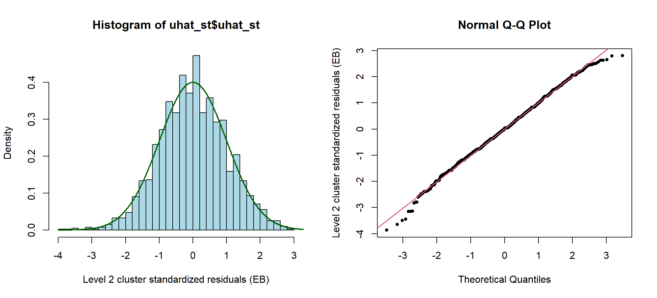
图 50.1: Standardized cluster level residuals (intercept) from the compound symmetry model
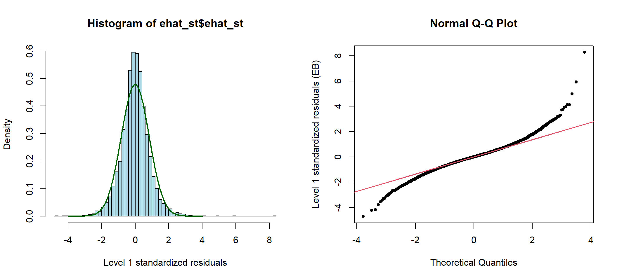
图 50.2: Standardized elementary level residuals from the compound symmetry model
混合对称模型的前提假设实在是太强了 (它假定个体内的方差保持不变,且个体间的协方差也保持不变)。你我都清楚,当考虑了时间以后,同一个体在时间上比较接近的点测量之间会更相似,也更相关。
50.2.2 随机参数模型 random intercept and slope model
实际上有多种方法可以放松混合对称模型对方差和协方差的约束性前提,其中之一是在随机截距模型中允许有随机斜率成分。
使用随机参数模型拟合纵向数据时的简单模型如下:
\[ Y_{ij} = (\beta_0 + u_{0j}) + (\beta_1 + u_{1j})t_i +e_{ij} \]
前一章讨论过(滚回49.5),这里随机参数模型的解释变量是时间\(t_i\),导致的结果之一是观测值的方差其实是随着时间变化而变化的(抛物线关系):
\[ \begin{aligned} \text{Var}(Y_{ij}) & = \text{Cov}(u_{0j} + u_{ij}t_i + e_{ij}, u_{0j} + u_{ij}t_i + e_{ij} ) \\ & = \sigma^2_{u_{00}} + \sigma^2_{u_{11}}t_i^2 + 2t_i\sigma_{u_{01}} + \sigma^2_e \end{aligned} \]
同时,同一患者不同时间测量的观测值之间的协方差是:
\[ \begin{aligned} \text{Cov}(Y_{1j}, Y_{2j}) & = \text{Cov}(u_{0j} + u_{1j}t_1 + e_{1j}, u_{0j} + u_{2j}t_2 + e_{2j}) \\ & = \sigma^2_{u_{00}} + \sigma^2_{u_{11}}t_1t_2 + \sigma_{u_{01}}(t_1 + t_2) \end{aligned} \]
不同患者任意测量时刻之间的协方差是:
\[ \begin{aligned} \text{Cov}(Y_{1j}, Y_{2j*}) & = \text{Cov}(u_{0j} + u_{1j}t_1 + e_{1j}, u_{0j*} + u_{2j *}t_2 + e_{2j*}) \\ & = 0 \end{aligned} \]
- Adult height measures 数据
利用上面的理论,来对身高数据拟合另一个混合效应模型:
# 对年龄中心化到以 26 岁为起点
hei_long <- hei_long %>%
  mutate(age = as.numeric(H_Age) - 26)
M_hei_ran <- lme(fixed = ht ~ age, random = ~ age | id, data = hei_long, method = "REML", na.action = na.omit)
#M_hei_ran <- lmer(ht ~ age + (age | id), data = hei_long, REML = TRUE)
summary(M_hei_ran)
## Linear mixed-effects model fit by REML
## Data: hei_long
## AIC BIC logLik
## 30382.43 30423.01 -15185.21
##
## Random effects:
## Formula: ~age | id
## Structure: General positive-definite, Log-Cholesky parametrization
## StdDev Corr
## (Intercept) 6.15885534 (Intr)
## age 0.05993187 -0.281
## Residual 1.25920202
##
## Fixed effects: ht ~ age
## Value Std.Error DF t-value p-value
## (Intercept) 162.49616 0.14113000 4416 1151.3934 0
## age -0.03158 0.00227368 4416 -13.8893 0
## Correlation:
## (Intr)
## age -0.279
##
## Standardized Within-Group Residuals:
## Min Q1 Med Q3 Max
## -3.938698652 -0.454242901 -0.006604401 0.429723565 5.505021425
##
## Number of Observations: 6397
## Number of Groups: 1980这个混合效应模型同时包含了随机截距和随机斜率两个部分。你可以用LRT 比较它和一个只有随机截距的模型哪个更好,但是我们没有办法比较它和混合对称模型哪个更优于拟合这个数据(因为他们的固定效应部分不同,在REML 方法下实际二者拟合的数据是不同的)。这个随机系数模型和前一个混合对称模型都给出了身高随着年龄增加而减少的相同结论。不同的是,随机系数模型把同一对象内不同时间观测值之间的等协方差的约束条件给放开了,因为用脚趾头想也知道同一个人不同时间测量的数据之间的协方差会随着时间跨度不同而发生改变。
根据随机系数模型给出的报告,计算模型估计的观测值 (身高的4个时间点) 的方差协方差矩阵:
\[ \begin{aligned} \hat{\text{Cov}}(Y_{1j}, Y_{2j}) & = \sigma^2_{u_{00}} + \sigma^2_{u_{11}}t_1t_2 +\sigma_{u_{ 01}} (t_1 + t_2) \\ & = 6.1588^2 + 0.0599^2t_1t_2 + (-0.28)\times6.1588\times0.0599 (t_1 + t_2)\\ & = 37.93 + 0.004\times t_2 \times t_2 - 0.104 \times(t_1 + t_2) \\ \hat{\text{Var}} (Y_1j) & = \sigma^2_{u_{00}} + \sigma^2_{u_{11}}t_1^2 - 2\sigma_{u_{01}}t_1 + \sigma_e^2 \\ & = 37.93 + 0.004 \times t_1^2 - 0.104\times2\times t_1 + 1.59 \end{aligned} \]
所以,当 \(t_1 = 0, t_2 = 10, t_3 = 17, t_4 = 27\) 时,
\[ \mathbf{\hat{\Sigma}_u} = \left( \begin{array}{cccc} 39.52 & 36.90 & 36.17 & 35.14 \\ 36.90 & 37.81 & 35.75 & 35.07 \\ 36.17 & 35.75 & 37.03 & 35.03 \\ 35.14 & 35.07 & 35.03 & 36.54 \\ \end{array} \right) \]
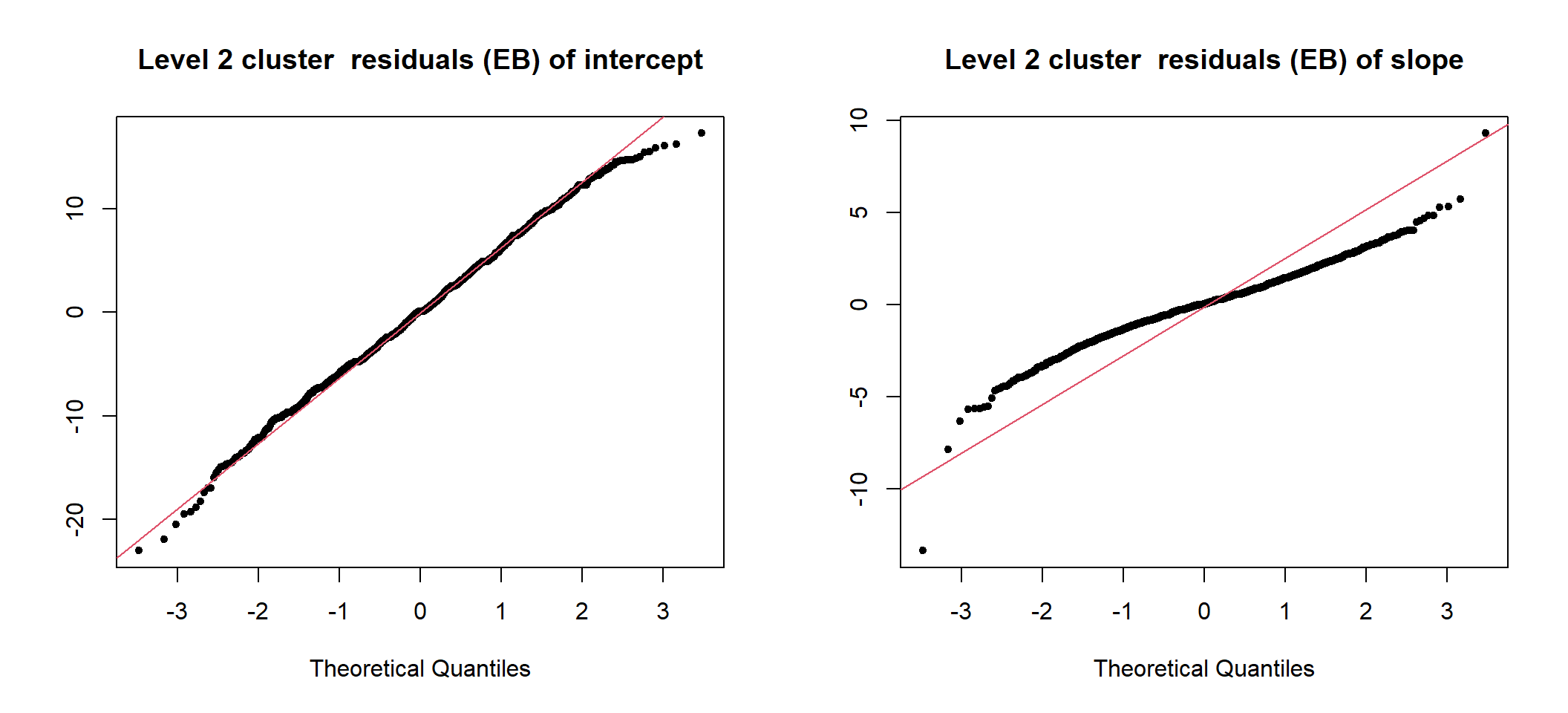
图 50.3: UN-Standardized cluster level residuals (intercept and slope) from the random intercept and slope model
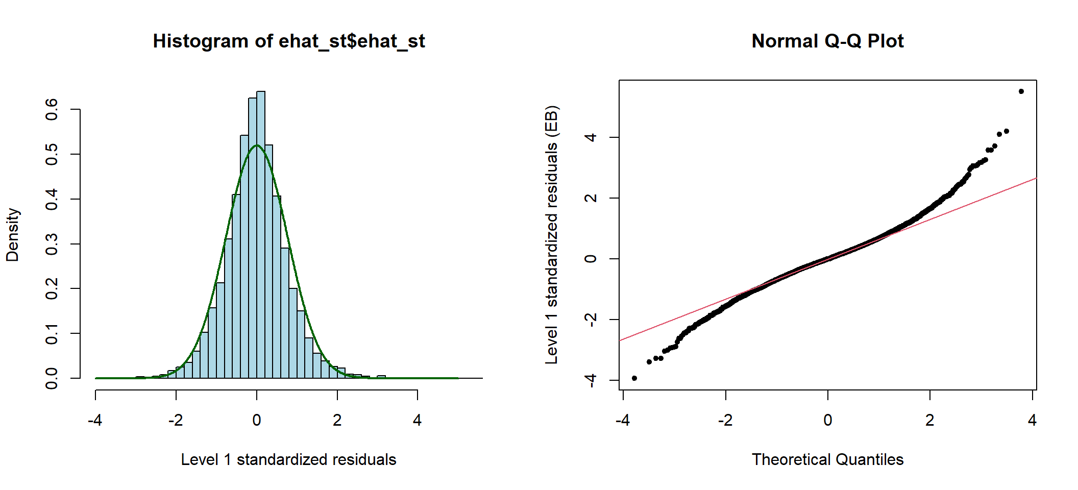
图 50.4: Standardized elementary level residuals from the random intercept and slope model
50.3 不固定测量时刻 variable occasions
当重复收集的数据不是平衡数据时,意味着不同的人数据的收集时间点不一样,我们就无法像前面那样用协方差矩阵的方式来描述不同人不同时间点之间测量值可能存在的相关性,也没有办法给每个时间点所有人的数据做平均值作为全部人的平均特质。
但是我们可以把不固定测量时刻的不平衡数据看作是受缺失值数据影响的平衡数据 (unbalanced data can be thought of as balanced data affected by missingness)。所以需要特别小心谨慎,因为用线性混合效应模型拟合这样的数据,其实是在含蓄地假设那些应该出现但是没有出现的测量值的缺失是随机的。
- Asian growth data 实例
在本部分开头的章节介绍过,这是一个收集了亚洲儿童在 6 周,8 个月,12 个月,和 27 个月大时的体重数据。
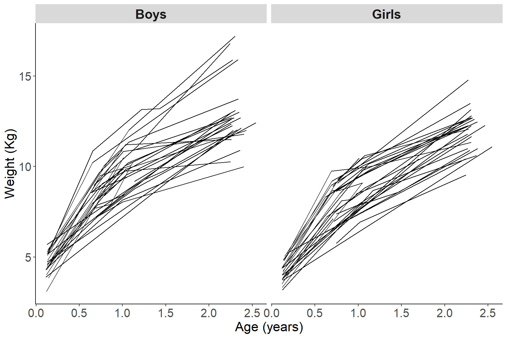
图 50.5: Growth profiles of boys and girls in the Asian growth data
如图 50.5 所示,观察男孩女孩的体重随着时间的变化,似乎暗示男孩子体重增加的速度较高,且男孩中体重增加的差异 (方差) 似乎也较女孩子的体重增加曲线来得大。另外,体重和年龄的关系并不是线性的,而且,这些数据中有缺失值。
50.3.1 随机截距模型
第一个想到的合适模型应该包括一个随机截距,一个固定效应的线性和抛物线性的年龄项,还有最后一个哑变量用以区分男孩和女孩:
\[ Y_{ij} = (\beta_0 + u_{0j}) + \beta_1t_{ij} + \beta_2 t_{ij}^2 + \beta_3 \text{girl}_j + e_{ij} \]
在 R 里拟合这个模型:
growth <- growth %>%
  mutate(age2 = age^2)

M_growth <- lme(fixed = weight ~ age + age2 + gender, random = ~ 1 | id, data = growth, method = "REML", na.action = na.omit)
summary(M_growth)
## Linear mixed-effects model fit by REML
## Data: growth
## AIC BIC logLik
## 565.9344 585.5416 -276.9672
##
## Random effects:
## Formula: ~1 | id
## (Intercept) Residual
## StdDev: 0.8594507 0.7394062
##
## Fixed effects: weight ~ age + age2 + gender
## Value Std.Error DF t-value p-value
## (Intercept) 3.799253 0.2121041 128 17.91221 0.0000
## age 7.817395 0.2905170 128 26.90856 0.0000
## age2 -1.705479 0.1089108 128 -15.65941 0.0000
## genderGirls -0.734137 0.2359099 66 -3.11194 0.0027
## Correlation:
## (Intr) age age2
## age -0.579
## age2 0.509 -0.970
## genderGirls -0.549 -0.009 0.008
##
## Standardized Within-Group Residuals:
## Min Q1 Med Q3 Max
## -2.32032124 -0.44485517 0.02407578 0.44611319 3.99180917
##
## Number of Observations: 198
## Number of Groups: 68## 由于样本量较小,这里如果使用极大似然法估计 ML,结果就和 REML 估计的随机效应的方差部分不太相同
M_growthml <- lme(fixed = weight ~ age + age2 + gender, random = ~ 1 | id, data = growth, method = "ML", na.action = na.omit)
summary(M_growthml)## Linear mixed-effects model fit by maximum likelihood
## Data: growth
## AIC BIC logLik
## 556.326 576.0556 -272.163
##
## Random effects:
## Formula: ~1 | id
## (Intercept) Residual
## StdDev: 0.8443385 0.7339017
##
## Fixed effects: weight ~ age + age2 + gender
## Value Std.Error DF t-value p-value
## (Intercept) 3.799744 0.2116025 128 17.956992 0.0000
## age 7.816195 0.2911648 128 26.844575 0.0000
## age2 -1.705076 0.1091520 128 -15.621112 0.0000
## genderGirls -0.734092 0.2346562 66 -3.128373 0.0026
## Correlation:
## (Intr) age age2
## age -0.582
## age2 0.511 -0.970
## genderGirls -0.548 -0.009 0.008
##
## Standardized Within-Group Residuals:
## Min Q1 Med Q3 Max
## -2.3409939 -0.4467712 0.0285789 0.4505660 4.0267069
##
## Number of Observations: 198
## Number of Groups: 6850.3.2 随机截距和斜率模型
此时我们再来用相同的数据拟合混合效应模型,现在允许线性年龄的斜率有随机变化:
M_growth_mix <- lme(fixed = weight ~ age + age2 + gender, random = ~ age | id, data = growth, method = "REML", na.action = na.omit)
summary(M_growth_mix)
## Linear mixed-effects model fit by REML
## Data: growth
## AIC BIC logLik
## 533.95 560.0929 -258.975
##
## Random effects:
## Formula: ~age | id
## Structure: General positive-definite, Log-Cholesky parametrization
## StdDev Corr
## (Intercept) 0.6148779 (Intr)
## age 0.5177688 0.135
## Residual 0.5741195
##
## Fixed effects: weight ~ age + age2 + gender
## Value Std.Error DF t-value p-value
## (Intercept) 3.795498 0.16814519 128 22.57274 0.0000
## age 7.698436 0.23985329 128 32.09644 0.0000
## age2 -1.657734 0.08859448 128 -18.71148 0.0000
## genderGirls -0.598384 0.19997480 66 -2.99230 0.0039
## Correlation:
## (Intr) age age2
## age -0.543
## age2 0.502 -0.929
## genderGirls -0.588 -0.008 0.007
##
## Standardized Within-Group Residuals:
## Min Q1 Med Q3 Max
## -2.04188399 -0.44260050 -0.03241251 0.41939982 2.66968194
##
## Number of Observations: 198
## Number of Groups: 68这里可以看到随机残差 (residuals) 的标准差 (StdDev) 部分在后者(混合系数模型)中明显变小了 \((0.74\rightarrow 0.54)\)。另外,第二层级残差和第一层级残差 (未标准化) 如图 50.6 和 50.7:
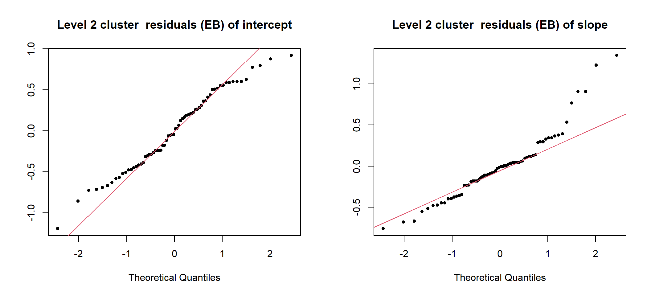
图 50.6: UN-Standardized cluster level residuals (intercept and slope) from the random intercept and slope model
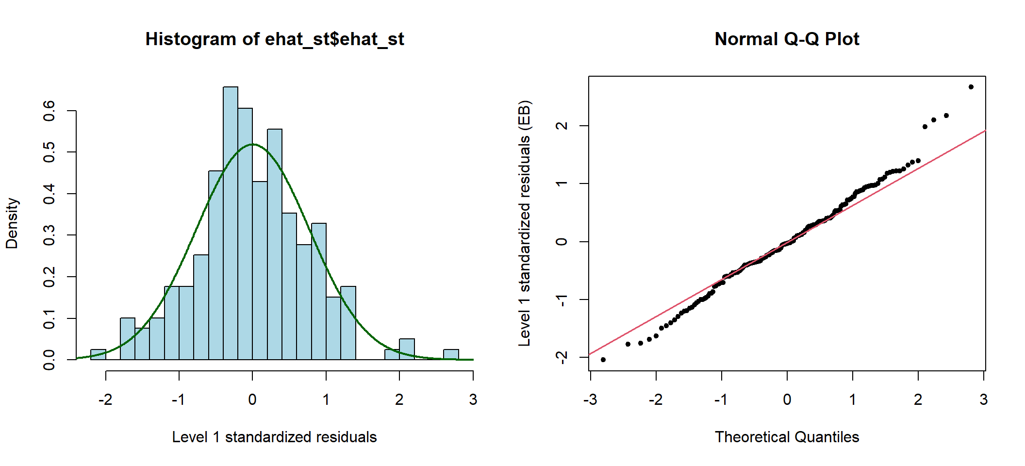
图 50.7: Standardized elementary level residuals from the random intercept and slope model
50.4 预测轨迹 predicting trajectories
比较只有随机截距模型,和随机系数模型给出的拟合曲线是否有差异 如图50.8,其实差异十分微小。可以用下面的 R 代码:
growth$traj2 <- fitted(M_growth_mix)
growth$traj1 <- fitted(M_growth)

G <- ggplot(growth[growth$id %in% c(258,1141,3148,287),], aes(x = age, y = weight)) + geom_point(shape = 19, size = 4) +
 # geom_line(aes(y = traj1)) +
#  geom_line(aes(y = traj2), linetype = 2) +
  stat_smooth(method = "lm", aes(y = traj1), formula = y ~ x + I(x^2), se = F, linetype = 2) +
  stat_smooth(method = "lm", aes(y = traj2), formula = y ~ x + I(x^2), se = F)  +
   theme(axis.text = element_text(size = 15),
  axis.text.x = element_text(size = 15),
  axis.text.y = element_text(size = 15)) +
  theme(axis.title = element_text(size = 17), axis.text = element_text(size = 8))


G +  facet_wrap( ~ id, ncol = 2) +
  theme(strip.text = element_text(face = "bold", size = rel(1.5)))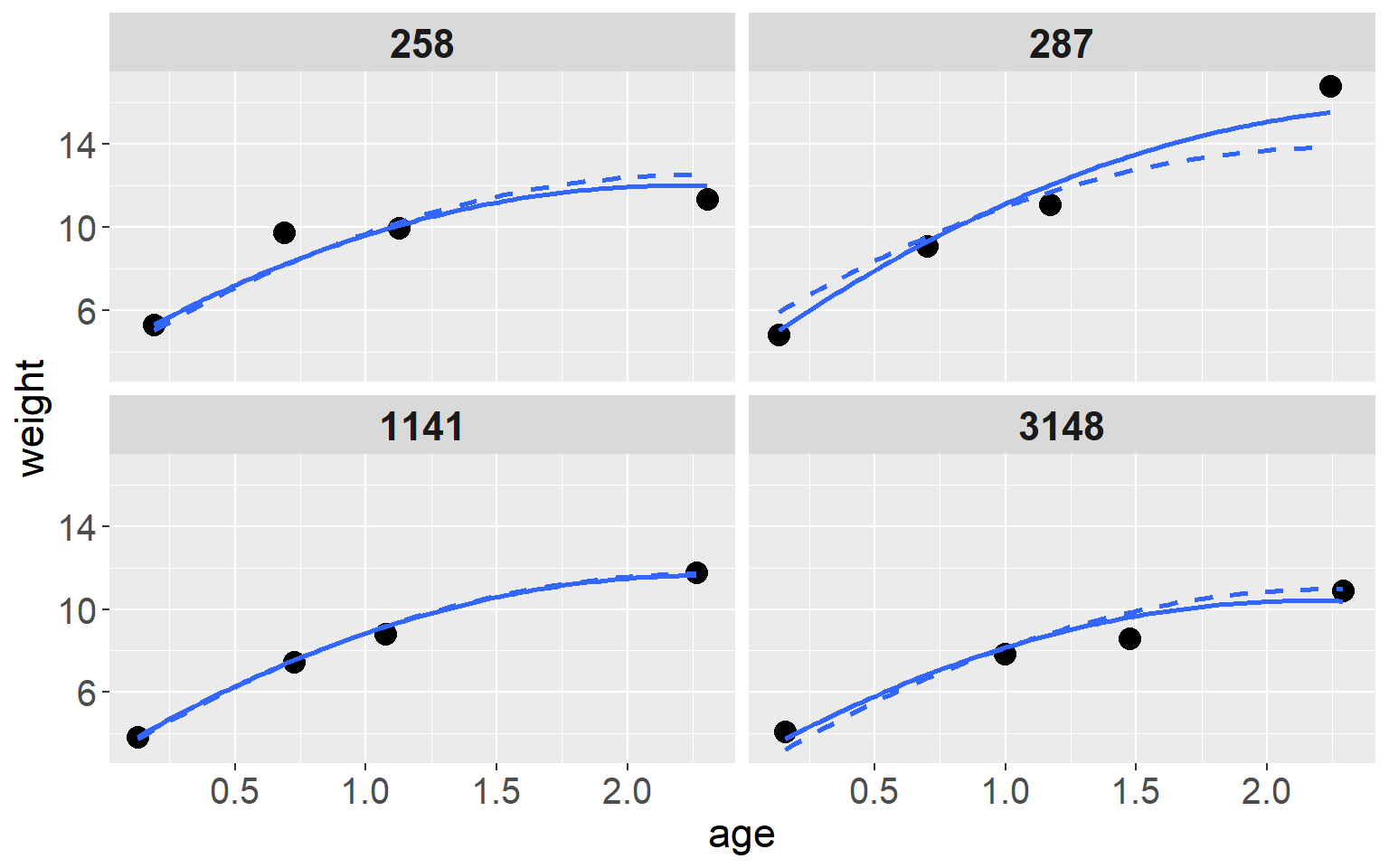
图 50.8: Observed weight and predicted growth profiles of four babies in the Asian growth data
50.5 多元混合效应模型矩阵标记法
50.5.1 边际结构 marginal structures
至此,我们接触过的各种混合效应模型其实代表的是数据不同的边际结构关系 (marginal relations)。
50.5.1.1 随机截距模型
纵向数据中,数据可能是平衡或不平衡数据,简单的随机截距模型可以标记如下:
\[ Y_{ij} = (\beta_0 + u_{0j}) + \beta_1 t_{ij} + e_{ij} \]
这个模型隐含着如下的条件关系 (conditional relation):
\[ \begin{aligned} Y_{ij} | t_{ij}, u_{0j} & \sim N(\beta_0 + \beta_1t_{ij} + u_{0j}, \sigma^2_e)\\ u_{0j}|t_{ij} & \sim N(0, \sigma^2_u) \\ \text{Var}(Y_{ij} | t_{ij}, u_{0j}) & = \sigma^2_e \end{aligned} \]
也就是说,观测值 \(Y_{ij}\) 以时间 \(t\),和随机截距 \(u_0\) 为条件的方差,只取决于 \(\sigma^2_e\)。所以,属于同一层(同一患者不同测量时间) 的测量值,以该层(患者) 的截距为条件(conditional on \(u_j\)) 的协方差是\(\text{Cov} (Y_{ij}, Y_{i*j}|t_{ij}, t_{i*j}, u_j) = 0\)。
\(Y_{ij}\) 针对 \(u_j\) 的边际期望 (marginal espectation with respect to \(u_j\)):
\[ E(Y_{ij}|t_{ij}) = \beta_0 + \beta_1 t_{ij} \]
其方差为\(\text{Var}(Y_{ij}|t_{ij}) = \sigma^2_u + \sigma^2_e\),同一层(同一患者) 的两个不同时刻测量值之间的边际协方差就是\(\text{Cov}(Y_{ij}, Y_{i*j}|t_{ij},t_{i*j}) = \sigma^2_u\)。
50.5.1.2 随机系数模型
模型的数学标记是
\[ Y_{ij} = (\beta_0 + u_{0j}) + (\beta_1 + u_{1j})t_{ij} + e_{ij} \]
等同于
\[ Y_{ij} = (\beta_0 + \beta_1t_{ij}) + (u_{0j} + u_{1j}t_{ij}) + e_{ij} \]
其条件关系是
\[ Y_{ij}|t_{ij},u_{0j},u_{1j} \sim N( \beta_0 + \beta_1t_{ij} + u_{0j} + u_{1j}t_{ij}, \sigma^2_e ) \]
其中, \(\mathbf{u}_j|t_{ij} \sim N(0, \mathbf{\Sigma}_u)\),且
\[ \mathbf{\sum}_{\mathbf{u}} =\left( \begin{array}{cc} \sigma^2_{u_{00}} & \sigma_{u_{01}} \\ \sigma_{u_{01}} & \sigma^2_{u_{11}} \\ \end{array} \right) \\ \text{Cov} (Y_{ij}, Y_{i*j}|t_{ij}, t_{i*j}, u_{oj}, u_{1j}) = 0 \]
其所指的\(Y_{ij}\)的边际分布:
\[ \begin{aligned} E(Y_{ij}|t_{ij}) & = \beta_0 + \beta_1t_{ij} \\ \text{Var}(Y_{ij}) & = \sigma^2_{u_{00}} +2\sigma_{u_{01}}t_{ij} + \sigma^2_{u_{11}}t_{ ij}^2 + \sigma^2_e \\ \text{Cov}(Y_{ij}, Y_{i*j}) & = \text{Cov}(u_{0j} + u_{1j}t_{ij} + e_{ij}, u_{0j} + u_{1j}t_{i*j} + e_{i*j}) \\ & = \sigma^2_{u_{00}} + \sigma_{u_{01}}(t_{ij} + t_{i*j}) + \sigma^2_{u_{11}}t_{ij}t_ {i*j} \text{ (for } i \neq i*) \\ \text{Cov}(Y_{ij}, Y_{i*j*}) & = \text{Cov}(u_{0j} + u_{1j}t_{ij} + e_{ij}, u_{0j* } + u_{1j*}t_{i*j*} + e_{i*j*}) \\ & = 0 \text{ (for } j \neq j*) \end{aligned} \]
也就是说同一层 (同一患者) 的不同测量值之间的协方差不为零,是时间的函数。
50.5.2 矩阵记法
如果数据本身是平衡数据,可以用如下的矩阵标记混合效应模型,
- \(j\) 是每个患者 (第二层级),\(\mathbf{Y}_j, \mathbf{e}_j\) 向量被定义为:
\[ \begin{aligned} \mathbf{Y}_j & = \left( \begin{array}{c} Y_{1j} \\ Y_{2j} \\ \cdots \\ \cdots \\ Y_{nj} \end{array} \right) \\ \mathbf{e}_j & = \left( \begin{array}{c} e_{1j} \\ e_{2j} \\ \cdots \\ \cdots \\ e_{nj} \end{array} \right) \\ \end{aligned} \]
用三次测量时间 \(t_1, t_2, t_3\) (以简便标记) 来继续接下来的推导,定义矩阵 \(\mathbf{T}, \mathbf{\beta}, \mathbf{u}_j\):
\[ \mathbf{T} = \left(\begin{array}{c} 1 & t_1 \\ 1 & t_2 \\ 1 & t_3 \end{array} \right) \\ \mathbf{\beta} = \left( \begin{array}{c} \beta_0 \\ \beta_1 \end{array} \right) \\ \mathbf{u}_j = \left(\begin{array}{c} u_{0j} \\ u_{1j} \end{array} \right) \]
如此经过利用定义好的向量,我们就可以把模型用矩阵标记来记录,从无穷无尽的下标中解放出来:
\[ \mathbf{Y = T\beta + Tu + e} \\ \text{Where } \mathbf{u} \sim N(0, \mathbf{\Sigma}_u) \\ \mathbf{e} \sim N(0, \sigma^2_e\mathbf{I}) \]
那么
\[ \text{Var}(\mathbf{Y}) = \mathbf{T\Sigma}_u\mathbf{T}^T + \sigma^2_e \mathbf{I} \]
50.5.3 混合效应模型的一般化公式
前面的例子用的虽然是时间做解释变量 (纵向数据),但是也可以推广到一般的混合效应模型:
\[ \mathbf{Y = T\beta + Zu + e} \]
其中 \(\mathbf{Z}\) 是类似 \(\mathbf{T}\) 的共变量矩阵。类似地,\(\mathbf{Y}\) 的方差是:
\[ \text{Var}(\mathbf{Y}) = \mathbf{Z\Sigma}_u\mathbf{Z}^T + \mathbf{\Sigma}_e \\ \mathbf{Y} \sim N(\mathbf{T\beta}, \mathbf{Z\Sigma}_u\mathbf{Z}^T + \mathbf{\Sigma}_e ) \]
这就是一个多元线性混合效应回归模型,大多数情况下,\(\mathbf{\Sigma}_e = \sigma^2_e\mathbf{I}\)。
50.5.4 其他可选择的方差协方差矩阵特征
学会了上面的矩阵标记以后,就应该了解在这样的多元混合效应模型中,对于层内方差,协方差矩阵的 \(\mathbf{\Sigma_u}\) 结构初步假设是相当重要的。目前为止我们接触过的模型的方差协方差矩阵结构列举如下 (为了简便标记都用\(3\times3\) 的矩阵来表示):
- 复合对称结构 (compound symmetry structure - compound symmetry model) 又名为可交换结构 (exchangeable structure)
\[ \mathbf{\sum}_{\mathbf{u}} =\left( \begin{array}{cc} \sigma^2_{u} + \sigma^2_e & \sigma^2_{u} & \sigma^2_{u} \\ \sigma^2_{u} & \sigma^2_{u} + \sigma^2_e& \sigma^2_{u} \\ \sigma^2_{u} & \sigma^2_{u} & \sigma^2_{u} + \sigma^2_e \\ \end{array} \right) \]
- 随机系数结构 random coefficient (RC) structure
\[ \mathbf{\sum}_{\mathbf{u}} =\left( \begin{array}{cc} \sigma^2_{u_{00}} + \sigma^2_e & \sigma^2_{u_{00}} + \sigma_{u_{01}} & \sigma^2_{u_{00}} + 2\sigma_ {u_{01}} \\ \sigma^2_{u_{00}} + \sigma_{u_{01}} & \sigma^2_{u_{00}} + 2\sigma_{u_{01}} + \sigma^2_{u_{11} } + \sigma^2_e& \sigma^2_{u_{00}} + 3\sigma_{u_{01}} + 2\sigma^2_{u_{11}} \\ \sigma^2_{u_{00}} + 2\sigma_{u_{01}} & \sigma^2_{u_{00}} + 3\sigma_{u_{01}} + 2\sigma^2_{u_{ 11}} & \sigma^2_{u_{00}} + 4\sigma_{u_{01}} + 4\sigma^2_{u_{11}}+\sigma^2_e \\ \end{array} \right) \]
除了这两个结构以外其他常见方差写方差结构还有:
- 自回归结构 (autoregressive structure):
\[ \frac{\phi}{1-\alpha^2} \left(\begin{array}{ccc} 1 & \alpha & \alpha^2 \\ \alpha & 1 & \alpha \\ \alpha^2 & \alpha & 1 \end{array} \right) \]
- 无固定结构 (unstructure):
\[ \left(\begin{array}{ccc} \sigma_{11} & \sigma_{12} &\sigma_{13} \\ \sigma_{21} & \sigma_{22} &\sigma_{23} \\ \sigma_{31} & \sigma_{32} &\sigma_{33} \end{array} \right) \]
最后不要忘记了还有完全独立结构 (不需要任何复杂模型或校正其数据间的依赖性):
\[ \sigma^2\left(\begin{array}{ccc} 1 & 0 & 0 \\ 0 & 1 & 0 \\ 0 & 0 & 1 \end{array} \right) \]
50.5.5 其他要点评论
各种结构模型之间的相互比较
- 似然比检验法 the likelihood ratio test (LRT)
前提是模型的固定结构不发生改变,两个嵌套式模型之间的比较是可以使用死然比检验的。缺点是统计学效能可能不太理想 (low power) - 模型的比较指标information criteria
就算是同一个数据,如果不同的协方差结构矩阵模型的固定效应部分也不同,似然比检验也不使用,这时候应该求助于赤池信息量(Akaike’s Information Criterion, AIC),或者贝叶斯信息量(Bayesian Criterion, BIC) 的比较。这两个信息量都是使用的模型的似然减去相应模型的参数数量作为评判标准。差别是 BIC 对参数的调整更加大些。但是,没人可以保证这些信息会永远相互认证,他们可能出现互相矛盾,也没人可以保证使用这些信息的比较可以证明你的模型是”最佳”模型。
- 似然比检验法 the likelihood ratio test (LRT)
50.6 第一层级的异质性 level 1 heterogeneity
目前为止,我们使用讨论过的模型,其实还默认另一个前提条件: 第一层级和第二层级的随机误差的方差是固定不变的 (level 1 and level 2 error variance are constant)。但是实际上我们可以把这个条件放宽,让模型允许第一层级随机误差的方差根据某个解释变量而不同,使得模型更加接近数据,这种模型被命名为复杂第一层级方差模型(complex level 1 variation)。下面继续使用 Asian growth data 来做说明。该数据测量了几百名亚洲儿童在0-3岁之间几个时间点的体重。现在我们来允许其第一层级 (每一个儿童在不同时间点测量的体重) 误差方差随着性别的不同而变化: \(\sigma_e = f(\text{gender})\)。这里的方程为了防止标准差变成负的而使用对数函数:
\[ \text{log} (\sigma_e) = \delta_1I_{\text{gender = boy}} + \delta_2I_{\text{gender=girl}} \]
这个加入了第一层级方差随机性的模型在 R 里可以这样拟合:
M_growth_l1 <- lme(fixed = weight ~ age + age2 + gender, random = ~ age | id, weights = varIdent(form=~1|gender), data = growth, method = "REML", na.action = na.omit)
summary(M_growth_l1)
## Linear mixed-effects model fit by REML
## Data: growth
## AIC BIC logLik
## 533.0603 562.4711 -257.5302
##
## Random effects:
## Formula: ~age | id
## Structure: General positive-definite, Log-Cholesky parametrization
## StdDev Corr
## (Intercept) 0.6449224 (Intr)
## age 0.4933637 0.129
## Residual 0.6422119
##
## Variance function:
## Structure: Different standard deviations per stratum
## Formula: ~1 | gender
## Parameter estimates:
## Boys Girls
## 1.0000000 0.7721288
## Fixed effects: weight ~ age + age2 + gender
## Value Std.Error DF t-value p-value
## (Intercept) 3.829412 0.17558114 128 21.80993 0.0000
## age 7.629728 0.23437556 128 32.55343 0.0000
## age2 -1.635069 0.08653522 128 -18.89484 0.0000
## genderGirls -0.604380 0.20451655 66 -2.95517 0.0043
## Correlation:
## (Intr) age age2
## age -0.523
## age2 0.471 -0.930
## genderGirls -0.630 0.011 0.008
##
## Standardized Within-Group Residuals:
## Min Q1 Med Q3 Max
## -1.97241108 -0.45150335 -0.06319209 0.46869701 2.95994617
##
## Number of Observations: 198
## Number of Groups: 68## Model df AIC BIC logLik Test L.Ratio p-value
## M_growth_l1 1 9 533.0603 562.4711 -257.5302
## M_growth_mix 2 8 533.9500 560.0929 -258.9750 1 vs 2 2.889701 0.089150.7 第二层级异质性 level 2 heterogeneity
我们还可以在模型中允许第二层级的结构不一样,这等同于认为这是一个三个层级的模型,其中第二层级分裂成男孩和女孩。
M_growth_l2 <- lme(fixed = weight ~ age + age2 + gender,
                   random = ~ age*gender | id,
                   data = growth, method = "REML", na.action = na.omit)
summary(M_growth_l2)
## Linear mixed-effects model fit by REML
## Data: growth
## AIC BIC logLik
## 539.9247 588.9425 -254.9623
##
## Random effects:
## Formula: ~age * gender | id
## Structure: General positive-definite, Log-Cholesky parametrization
## StdDev Corr
## (Intercept) 0.5567034 (Intr) age gndrGr
## age 0.6945150 0.037
## genderGirls 0.8535854 -0.552 -0.003
## age:genderGirls 0.7253379 -0.095 -0.948 0.131
## Residual 0.5694754
##
## Fixed effects: weight ~ age + age2 + gender
## Value Std.Error DF t-value p-value
## (Intercept) 3.820437 0.1601151 128 23.86057 0.0000
## age 7.614974 0.2351766 128 32.37982 0.0000
## age2 -1.646424 0.0874516 128 -18.82669 0.0000
## genderGirls -0.608823 0.2031867 66 -2.99637 0.0038
## Correlation:
## (Intr) age age2
## age -0.543
## age2 0.520 -0.945
## genderGirls -0.531 -0.048 0.011
##
## Standardized Within-Group Residuals:
## Min Q1 Med Q3 Max
## -2.024047990 -0.439995806 -0.009544513 0.456496526 2.743961402
##
## Number of Observations: 198
## Number of Groups: 68growth <- growth %>%
mutate(boy = as.numeric(gender == "Boys"),
girl = as.numeric(gender == "Girls")) %>%
mutate(age_boy = age*boy,
age_girl = age*girl)
#M <- lmer(weight ~ age + age2 + girl + (age_boy |id) + (age_girl| id), data = growth, REML = TRUE)
#growth <- growth %>%
# mutate(boy = ifelse(gender == "Boys", 1, 0),
# girl = ifelse(gender == "Girls", 1, 0),
# age_boy = age*boy,
# age_girl = age*girl)
#M_growth_l22 <- lme(fixed = weight ~ age + age2 + girl,
# random = list( ~ girl + age_girl | id,
# ~ boy + age_boy | id),
# data = growth, method = "REML", na.action = na.omit)
#summary(M_growth_l22)
M_growth <- lme(fixed = weight ~ age + age2 + gender, random = ~ age|id, data = growth, method = "REML",na.action = na.omit)
anova(M_growth_l2, M_growth)## Model df AIC BIC logLik Test L.Ratio p-value
## M_growth_l2 1 15 539.9247 588.9425 -254.9623
## M_growth 2 8 533.9500 560.0929 -258.9750 1 vs 2 8.025378 0.330450.8 分析策略
进行统计建模之前,请思考你想从数据中探寻什么问题的答案?
- 是想了解某一个共变量在层内 (同一个体不同时间,或者统一学校不同学生之间) 的条件效应 (conditional effect)?
- 是想探索层内和层间数据的变化程度?
- 是想了解一个共变量的边际效应 (marginal effect) 吗?
如果是 1 或 2 两个问题的话,请使用混合效应模型。如果是 1,但是那个共变量却不是定义于层水平的,那就只好放弃回到简单的固定效应模型。如果是 3,需要考虑使用 GEE。
50.8.1 模型选择和建模步骤
详细请参考 (Verbeke 1997)。
当拟合一个混合效应模型时,意味着均值的结构和协方差的结构可以被确定 (an appropriate mean structure as well as covariance structure is specified)。协方差结构,解释了均值结构无法解释的数据随机变化,所以二者之间彼此高度互相依赖。另外,适当的协方差模型对于用数据进行人群参数的有效统计推断过程是必不可少的。
- 第一步:
由于固定效应部分不能完美解释数据的变异,所以协方差结构就是用来辅助解释这部分数据变异的辅助工具。建模的起点就应该是,先建立一个饱和 (甚至是过饱和 overelaborated) 的模型给均值结构 (固定效应部分),从而确保之后要增加的随机效应部分不受固定效应部分的拟合错误影响。所以,开始建模时,要先把所有可能考虑到的固定效应全部加入模型中去 (包括连续变量的二次方形式/或其他非线性关系,包括所有变量之间的交互作用)。这样做其实是使用过度饱和的参数使得均值结构在模型中尽量在后面加入随机效应之前保持不变。在可选的那些数据结构中,我们也应当考虑到数据中不同层级结构可能存在的异质性。要注意的是,随机效应部分,不能也不应该在没有把所有可能的一次方程结构都考虑进去之后(a random effect for the linear effect of time),就上马二次方程/或更高次方程的随机效应(a random effect for the quadratic effect of time)。 然后我们把饱和模型的残差(residuals),异常值(outliers),拟合值(fitted values),和可能的(potential) 随机效应模型作出的这些残差,异常值,拟合值之间进行比较。
- 第二步:
一旦你在饱和模型的条件下,确认好了随机效应应该有的形式,接下来就是逐步精简模型固定效应部分的过程:
- 用 Wald 检验 (当使用 REML 时),或者 LRT (使用 ML 时) 来精简化固定效应部分。
- 反复检查残差,异常值,以及拟合值跟观测值
- 使用模型的预测轨迹和观测值的点做视觉比较
- 用人话把你的模型解释给老奶奶听懂