第 46 章相互依赖数据及简单的应对方案

46.1 相互依赖的数据

线性回归模型，广义线性回归模型，他们背后都有一个十分十分十分重要的假设–数据的相互独立性。这个前提假设常常会在现实数据中得不到满足，因为数据与数据之间在背后很可能会有有所关联，也许是已知的，也许是未知的因素让某些数据显得更加接近彼此。这个章节，主要的内容就是举例说明分层数据在日常生活中的常见性，以及处理这个非独立性质的必要性。

图 46.1 展示的箱式图显示的是六个不同医院对各自 12 名患者收缩期血压测量的结果。如果把医院看做一个单位，取院内患者的平均值，那么六所医院的血压均值最大为 135.7 mmHg，最小是 117.7 mmHg，六所医院测量的血压总体均值为 125.6 mmHg。

## ── Attaching core tidyverse packages ──────────────────────── tidyverse 2.0.0 ──
## ✔ dplyr     1.1.3     ✔ readr     2.1.4
## ✔ forcats   1.0.0     ✔ stringr   1.5.0
## ✔ lubridate 1.9.3     ✔ tibble    3.2.1
## ✔ purrr     1.0.2     ✔ tidyr     1.3.0
## ── Conflicts ────────────────────────────────────────── tidyverse_conflicts() ──
## ✖ dplyr::filter()     masks stats::filter()
## ✖ dplyr::group_rows() masks kableExtra::group_rows()
## ✖ dplyr::lag()        masks stats::lag()
## ℹ Use the conflicted package (<http://conflicted.r-lib.org/>) to force all conflicts to become errors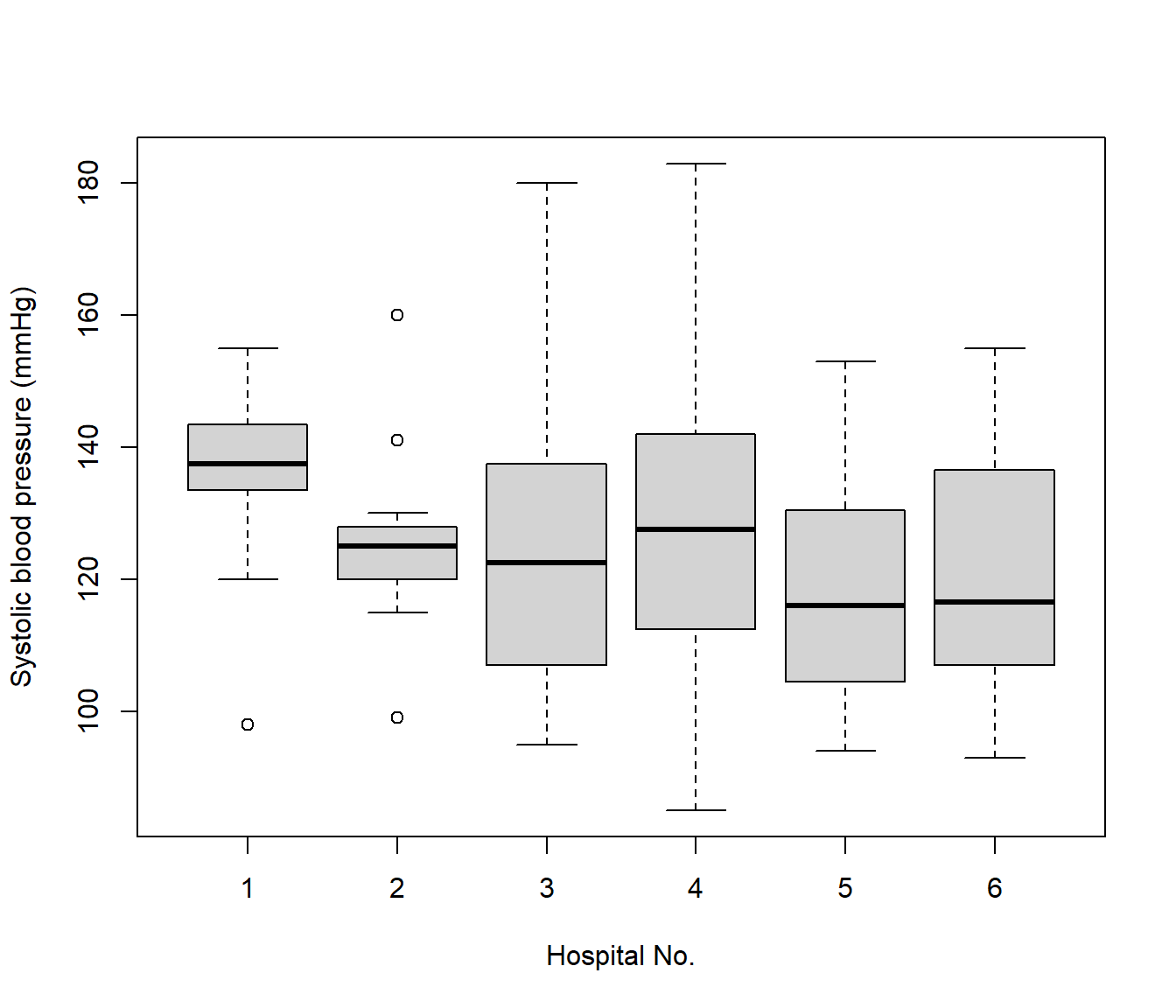

图 46.1: Box and whiskers plot of measured SBP in patients from six hospitals

图 46.2 展示的是对 17 名患者使用两种不同的测量方法测量的最大呼吸速率 (peak-expiratory-flow rate, PEFR)。两种方法又测量了两次，途中展示的是其中一种测量方法前后两次测量结果的散点图。

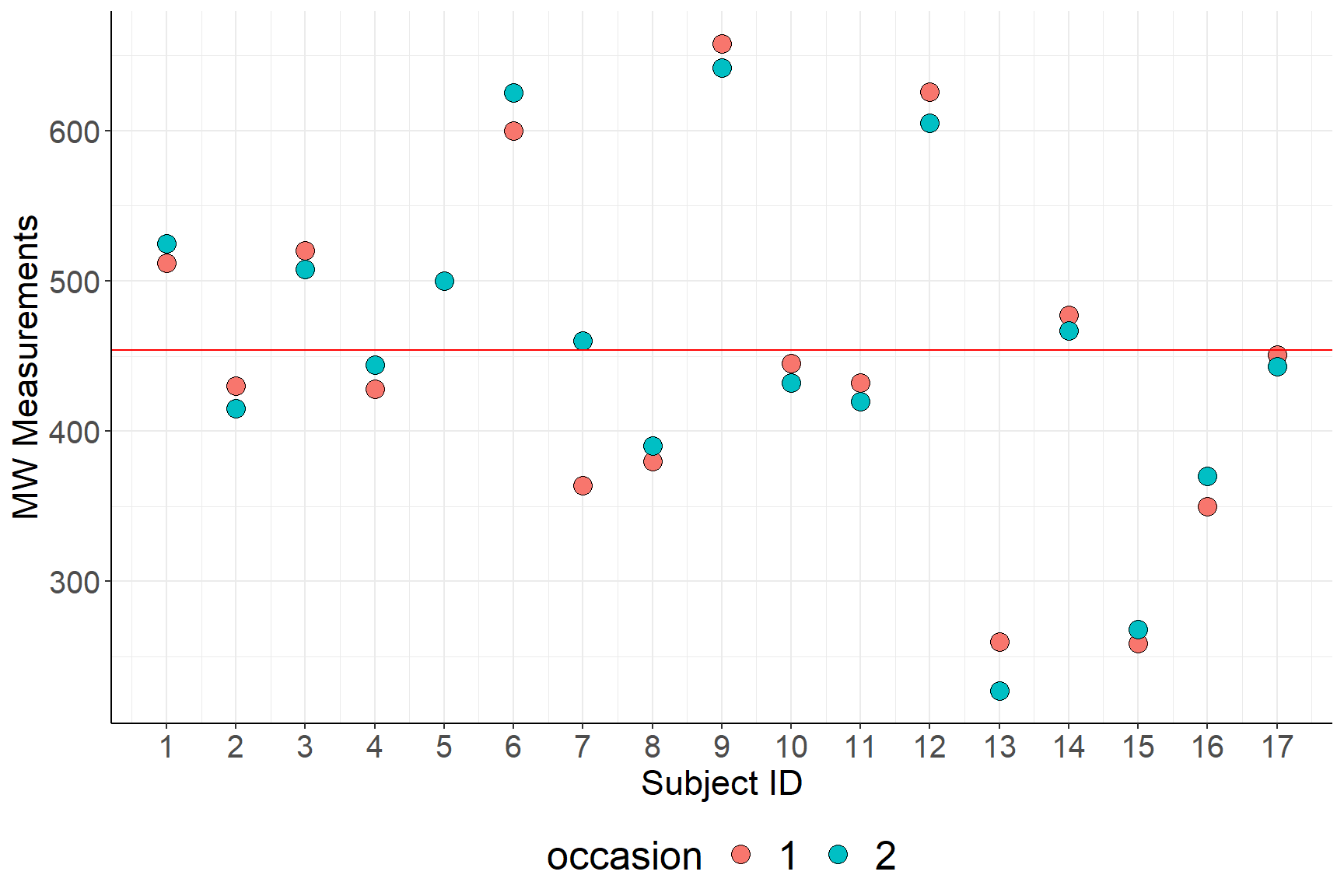
图 46.2: Two recordings of PEFR taken with the Mini Wright meter

图 46.3 展示的来自全英 65 所学校的 4059 名学生入学前阅读水平测试成绩 (LRT) 和毕业时 GCSE 考试成绩之间的散点图关系。值得注意的是该图其实无视了学校这个变量，把每个学生看成相互独立的个体。但是当我们随机选取四所学校，看它们各自的学生的成绩表现 (图 46.4)。很显然，之前忽视了学校这一层级的变量是不恰当的，因为不同学校学生的入学前和毕业时成绩之间的相关性很明显存在不同的模式(四所学校的回归线各自的截距和斜率各不相同)。

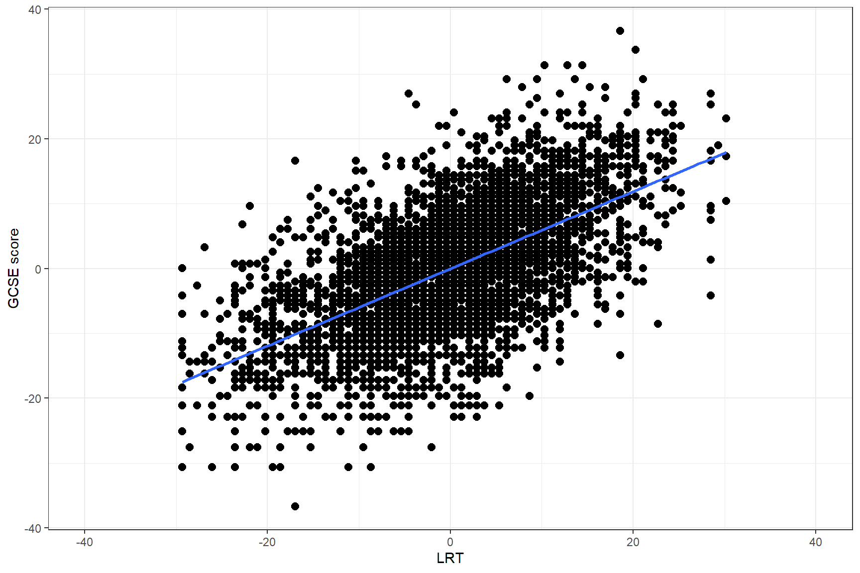
图 46.3: GCSE by LRT in all 65 schools

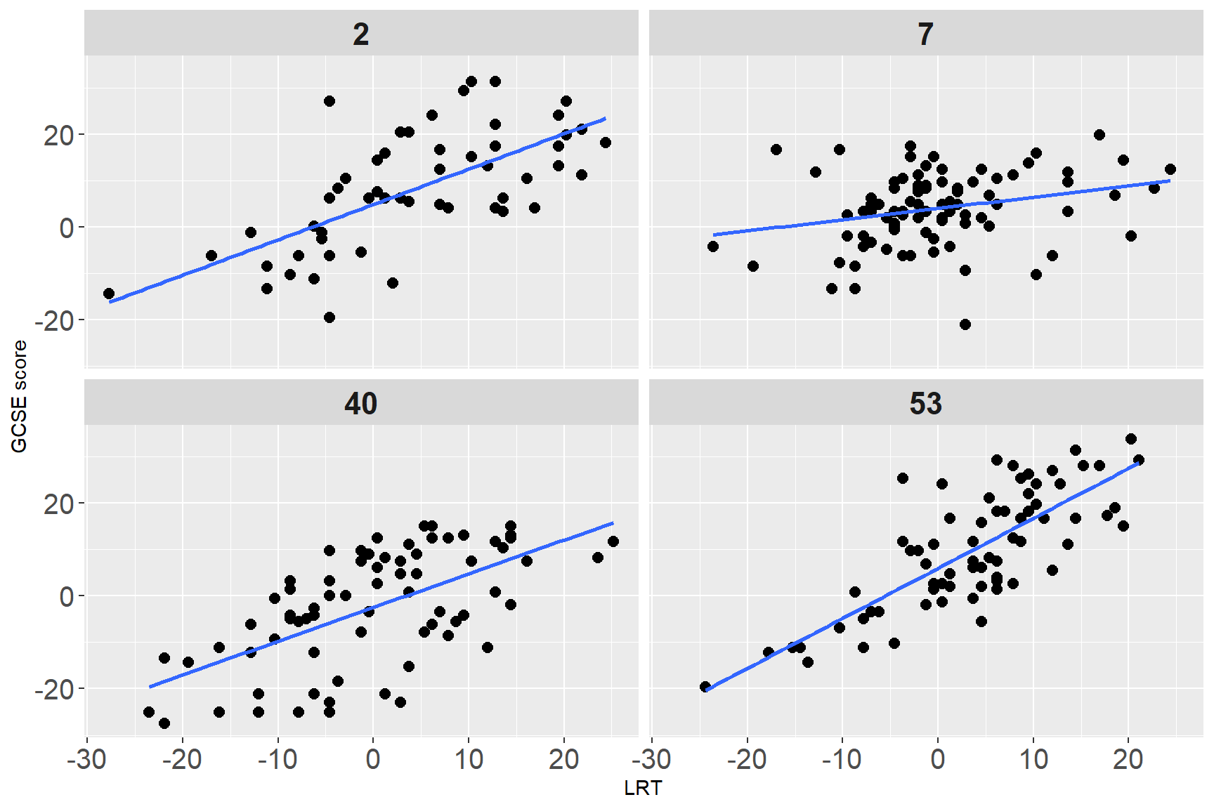
图 46.4: GCSE by LRT in four randomly selected schools

另一个特别好的例子展示在图 46.5 中，是关于同一个母亲的不同孩子的出生体重的数据。一个母亲可以有多个孩子，每个母亲的孩子之间的出生体重很明显无法看作相互独立。图中展示的是，3300 名生了两个孩子的母亲的孩子们出生体重的散点图。同一个母亲的小孩用线相连。显然，同一个母亲生的孩子，其出生体重比不同母亲的孩子出生体重差距更小，更接近彼此，因为他们来自同一个母亲。可以想象，一个母亲如果身材高大，那么她的孩子们可能都倾向于有比较高的出生体重。所以同一个母亲的孩子之间体重是有相关关系的 (within correlation)。

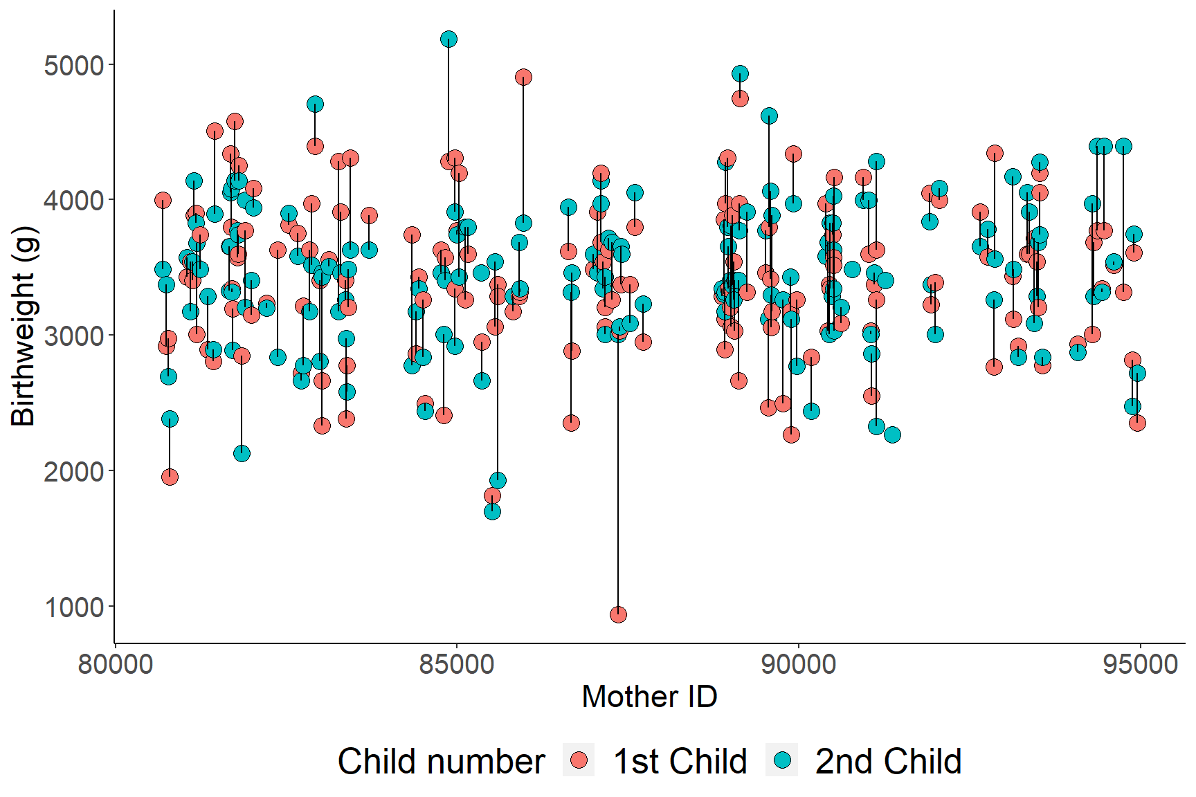
图 46.5: Birthweight of siblings by maternal identifier

最后一个用于本章节的实例是，一项研究亚洲儿童生长状况的调查分别记录了 198 个数据点，68 个儿童在 0 到 3 岁之间的四个年龄点的体重数据。图 46.6 展示的就是这个典型的随访数据的个人生长曲线。且图中每个人的生长轨迹提示，男孩子的生长过程可能相互之间体重差异显得较女孩子来得大。如果，我们用每个儿童自己的数据，给每个儿童拟合各自的回归线，数据显然不足，但是如果我们决定忽略个体的生长的随机效应 (不均一性)，又显得十分不妥当。

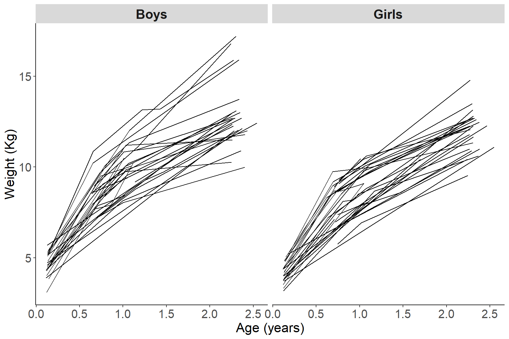
图 46.6: Growth profiles of boys and girls in the Asian growth data

上述例子中的数据，均提示我们数据与数据之间独立性的假设，常常会遇到尴尬的局面。因为数据与数据之间本身就不可能完全独立。

同一个诊所或者医院的患者，他们之间可能有着某些相似的因素从而导致他们的血压相比其他医院的人彼此更加接近。这个原因可能是有同一家医院的患者可能有类似的疾病。
同一患者身上反复抽取样本，也就是说一个对象贡献了多个数据的时候，这些来自同一对象的数据当然具有相对不同对象数据更高的均质性。
同一所学校的学生的成绩或内部的相关性，很可能大于不同学校两个学生之间成绩的相关性。因为同一学校的孩子可能共享某些共同的特征，比如说相似的家庭经济背景，或者是同样的教学内容教学老师等环境因素。这样，来自同一所学校的孩子的成绩很可能就会更加相似。
至于说家庭数据就更加典型了。来自同一家庭的兄弟姐妹，有着极强的相关性，因为他们共享着遗传因素，或者是相似的家庭教育/饮食/生活习惯等环境因素。
同一个体身上的纵向 (时间) 随访数据很显然会比不同患者有更强的内部相关性。

目前位置介绍的这些常见实例中，可以发现它们有一个共通点。就是这些数据其实内部是有分层结构的 (hierarchy)。这些数据中，都有一个最底层单元 (elementary units/level 1)，还有一个聚合单元 (aggregate units/level 2)，聚合单元常被命名为层级 (cluster)。

表 46.1: Hierarchy in the data (5 examples in Chapter 1)
Level
Aggregate	Elementary
hospitals	patients
individuals	PEFR measures
schools	pupils
mothers	children
children	visits

正如表格 46.1 总结的那样，这些数据中存在这层级结构，这种数据被称为分层数据 (hierarchical)，或者叫嵌套式数据 (nested data)。根据你所在的知识领域，它可能还被命名为多层结构数据 (multilevel and clustered data)。在一些研究中，你可能会遇见从实验设计阶段就存在分层结构的数据，比如使用分层抽样 (multistage sampling) 的设计的实验等。这样的实验设计最常在人口学，社会学的研究中看到。在大多数医学研究中，每个数据点(observation point, level 1)，所属的层(cluster) 本身可能是我们感兴趣的研究点(例如同属于一个家庭，相同母亲的后代)，又或者是同一个人/患者的随着时间推移的随访健康状态(如生长曲线，体重变化，疾病康复情况)。

如果用前面用过的图46.6 的生长曲线做例子，那么每个被调查的儿童，就是该数据的第二级层，每个随访时刻测量的体重数据，则是观察的数据点。这个数据还有一个特点是，观察数据点是有前后的 (时间) 顺序的，这是一个典型的纵向研究数据 (longitudinal data)。

46.2 数据有依赖性导致的结果

如果你手头的数据，结构上是一种嵌套式结构数据，那么任何无视了这一点作出的统计学推断都是有瑕疵的。相互之间互不独立这一特质，需要通过一种新的手段，把嵌套式的数据结构考虑进统计学模型里来。

在一些情况下，数据的嵌套式结构可能可以被忽略掉，但是其结果是导致统计学的估计变得十分低效 (inefficient procedure)。你可能会听说过一般化估计公式 (generalized estimating equations)，是其中一种备择手段，因为在这一公式中，你需要人为地指定数据与数据之间可能的依赖关系是怎样的。

其实，即使有人真的在分析过程中忽略了数据本身的嵌套式结构，他会发现最终在描述分析结果的时候，还是无法避免这一严重的问题。另外一些统计学家可能记得在稳健统计学法中，三明治标准误估计法也是可以供选择的一种处理相关数据的手段。

46.3 边际模型和条件模型 marginal and conditional models

边际模型和条件模型的概念其实不是分层模型特有的，却在分析分层数据模型时十分有用。假如，对于某个结果变量 $Y$ 有它如下的回归模型，其中我们把某个单一的共变量 $Z$ 从模型中分离出来，加以特别关注:

\[ g\{ \text{E}(Y|\textbf{X},Z) \} = \beta\textbf{X} +\gamma Z \]

这是一个典型的条件模型，它描述了结果变量 $Y$ 的期望是以怎样的条件和解释变量 $\textbf{X},Z$ 之间建立关系的。每个解释变量的回归系数，其含义都是以其他同一模型中的共变量不变的条件下，和结果变量之间的关系。经过这样的解读，你会知道，其实本统计学教程目前为止遇见过的所有的回归模型都是条件模型。如果此时我们反过来思考，把上述模型中单独分离出来的单一共变量$Z$ 对于结果变量$Y$ 均值的影响合并起来(对共变量$Z$ 积分即可)，此时我们得到的就是共变量$\textbf{X}$ 和结果变量$Y$ 之间，关于$Z$ 的边际模型(Marginal model):

\[ \text{E}_Z\{ \text{E}(Y|\textbf{X}, Z) \} = \text{E}_Z\{ g^{-1}(\beta\textbf{X} + \gamma Z) \} \\ \text{Where } \text{E}(Z) = 0 \]

用线性回归来举例:

\[ \text{E}(Y| \textbf{X}, Z) = \beta\textbf{X} + \gamma Z \]

那么此时共变量 $\textbf{X}$ 的边际模型回归系数 $\beta$ 的含义，和条件模型时的回归系数其实是相同的含义:

\[ \text{E}_Z\{\text{E}(Y|\textbf{X},Z)\} = \text{E}_Z(\beta\textbf{X} + \gamma Z) = \beta\ textbf{X} + \gamma\text{E}(Z) = \beta\textbf{X} \]

为什么这里的边际模型对于分层数据来说很重要呢？答案在于，嵌套式数据中，我们常常关心那第二个阶层(重复测量某个指标的患者，学生成绩数据中的学校层级，等) 在它所在的那个阶层中和结果变量之间的平均关系。

表 46.2: Example data
Cluster (j)	id (i)	X	Y	X	Y
1	1	1	5	2	6
1	2	3	7	2	6
2	1	2	4	3	5
2	2	4	6	3	5
3	1	3	3	4	4
3	2	5	5	4	4
4	1	4	2	5	3
4	2	6	4	5	3
5	1	5	1	6	2
5	2	7	3	6	2

46.3.1 标记法 notation

$Y_{ij}$ 标记第 $j$ 层的第 $i$ 个个体;
$i = 1, \cdots, n_j$ 表示第 $j$ 层中共有 $n_j$ 个个体 (elements);
$j = 1, \cdots, J$ 表示数据共有 $J$ 个第二阶层 (clusters);
$N = \sum_{j=1}^J n_j$ 表示总体样本量等于各个阶层样本量之和;
特殊情况: 如果每个阶层的个体数相同 $n$，$N=nJ$，这样的数据被叫做均衡数据 (balanced data)。

46.3.2 合并每个阶层

过去常见的总结嵌套式数据的手段只是把每层数据取平均值，这样的方法简单粗暴但是偶尔是可以接受的，只要你能够接受如此处理数据可能带来的如下后果:

各层数据均值，其可靠程度 (方差) 随着各层的样本量不同而不同 (depends on the number of elementary units per cluster);
变量的含义发生改变。如果是使用层水平(cluster level) 的数据，本来测量给个体的那些变量，就变成了层的变量，从此作出的任何统计学推断，只能限制在层水平(ecological fallacy, as correlations at the macro level cannot be used to make assertions at the micro level);
由于无视了层内个体数据，导致大量信息损失。

此处我们借用 (Snijders and Bosker 1999) 书中第 28 页的人造数据，如下表

Artificial data
Cluster $(j)$	id $(i)$	$X$	$Y$	$\bar{X}$	$\bar{Y}$
1	1	1	5	2	6
1	2	3	7	2	6
2	1	2	4	3	5
2	2	4	6	3	5
3	1	3	3	4	4
3	2	5	5	4	4
4	1	4	2	5	3
4	2	6	4	5	3
5	1	5	1	6	2
5	2	7	3	6	2

这个表中的人造数据，其结构是一目了然的，它的第二层级数量是 5，每层的个体数量是 2。这是一个平衡数据。由于这是个我们人为模拟的数据，图 46.7 也显示它没有随机误差，所有数据都在各自的直线上。

dt <- read.csv("../backupfiles/hierexample.csv", header = T)
names(dt) <- c("Cluster", "id", "X", "Y", "Xbar", "Ybar")
dt$Cluster <- as.factor(dt$Cluster)
##ggthemr('fresh')

ggplot(dt, aes(x = X, y = Y, shape = Cluster, colour = Cluster)) + geom_point(size =5) +
  theme(axis.text = element_text(size = 15),
  axis.text.x = element_text(size = 15),
  axis.text.y = element_text(size = 15)) +
  labs(x = "X", y = "Y")  +
  theme(axis.title = element_text(size = 17), axis.text = element_text(size = 8)) + 
theme(legend.position = "bottom", legend.direction = "horizontal") + theme(legend.text = element_text(size = 19), legend.title = element_text(size = 19))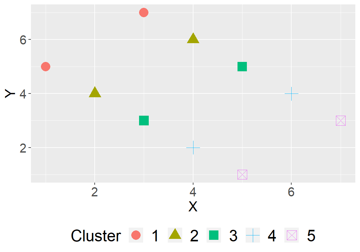

图 46.7: Artificial data: scatter of clustered data

如果我们无视其分层数据的嵌套式结构，把每个数据都看作是独立的样本，拟合一个整体回归 (total regression) 图 46.8:

\[ \hat Y_{ij} = 5.33 - 0.33 X_{ij} \]

##ggthemr('fresh')

ggplot(dt, aes(x = X, y = Y)) + geom_point(size = 5, shape = 23) + 
  geom_smooth(method = "lm", se = FALSE, linetype = 2) +
  theme(axis.text = element_text(size = 15),
  axis.text.x = element_text(size = 15),
  axis.text.y = element_text(size = 15)) +
  labs(x = "X", y = "Y")  +
  theme(axis.title = element_text(size = 17), axis.text = element_text(size = 8)) + 
theme(legend.position = "bottom", legend.direction = "horizontal") + theme(legend.text = element_text(size = 19), legend.title = element_text(size = 19))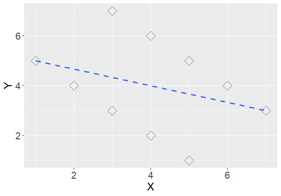

图 46.8: Artificial data: Total regression

如果我们只保留层级数据本身，求了变量$X,Y$ 在每层的均值的话，就得到了层间回归(between regression) 图46.9 – 变量$ X,Y$ 之间的回归直线的斜率变得更大了:

\[ \hat{\bar{Y}}_j = 8.0 - 1.0 \bar{X}_j \]

##ggthemr('fresh')

ggplot(dt, aes(x = X, y = Y)) + geom_point(size =5, shape=23) + 
    geom_smooth(method = "lm", se = FALSE, linetype = 2) +
  geom_abline(intercept = 8, slope = -1) + 
  geom_point(aes(x = Xbar, y=Ybar, size = 5)) +
  theme(axis.text = element_text(size = 15),
  axis.text.x = element_text(size = 15),
  axis.text.y = element_text(size = 15)) +
  labs(x = "X", y = "Y")  +
  theme(axis.title = element_text(size = 17), axis.text = element_text(size = 8)) + theme(legend.position="none")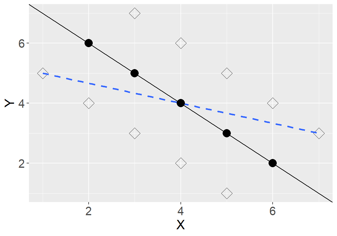

图 46.9: Artificial data: scatter of clustered data

46.3.3 生物学悖论 ecological fallacy

生物学悖论常见于我们认为某分层数据中层级变量之间的关系，同样适用与层级中的个体之间: 例如比较A 国和B 国之间心血管疾病的发病率，发现A 国国民食盐平均摄入量高于B 国，很多人可能就会下结论说食盐摄入量高的个体，心血管疾病发病的危险度较高。然而，这样的推论很多时候是错误的。

曾经在 (W. S. Robinson 1950) 论文中举过的著名例子: 该研究调查美国每个州的移民比例，和该州相应的识字率之间的关系。研究者发现，移民比例较高的州，其识字率也较高 (相关系数 0.53)。由此就有人下结论说移民越多，那个州的教育水平会比较高。但是实际情况是，把每个个体的受教育水平和该个体本身是不是移民做了相关系数分析之后发现，这个关系其实是负相关 (-0.11)。所以说在州的水平作出的统计学推断-移民多的州受教育水平高-是不正确的。之所以在州水平发现移民比例和受教育水平之间的正关系，是因为移民倾向于居住在教育水平本来就比较高的本土出生美国人的州。

46.3.4 分解层级数据

如果是分析最初层级数据 (level 1) 的话，我们还需要考虑下列一些问题:

当心数据被多次利用

如果我们关心的变量其实是在第二层级的(level 2/cluster level)，但是你却把它当作是第一层级的数据，就会引起数据很多的错觉，因为同一层的个体他们的层属变量都是一样的，你拥有的数据其实并没有你想的那么多。

前文中用过的GCSE 数据其实是一个很好的例子，下表中归纳了调查的学校类型(男校，女校或者混合校)，以及按照每个学生个人所属学校类型的总结，可以看出，当你尝试使用个人(elementary level) 水平的数据分析实际上是第二层级数据的特性时，你会被误导。因为个人数据告诉你， 34% 的学生在女校学习，然而正确的分析法应该是，学校中有 31% 的学校是女校。

表 46.3: Aggregated and disaggregated
School type	Cluster Level		Elementary Level
X	N	X.	N.1	X..1
mixed	35	54	2169	53
boys only	10	15	513	13
girls only	20	31	1377	34
Total	65	100	4059	100

分层数据分析法

有人会说，既然如此，那么我们就把数据放在每层当中分析就好了 (stratified analyses)。还是用前文中用过的人造 5 层数据来说明这样做的弊端。前面用了两种方法 (total regression, between regression) 来总结这个 5 层的人造数据 46.9。最后一种分析此数据的方法是，把 5 层数据分开分别做回归线如图 46.10。等同于我们的对数据拟合五次下面的回归方程:

\[ \hat Y_{ij} - \bar{Y}_j = \beta(X_{ij} - \bar{X}_j) \]

这种模型被叫做层内回归 (within regression)。这 5 个线性回归的斜率都是 1，是五条不同截距的平行直线。因为我们自己编造的数据的缘故，现实数据不太可能恰好所有层内回归的斜率都是完全相同的。这其实也是曾内回归法的一个默认前提 – 每层数据中解释变量和结果变量之间的关系是相同的。

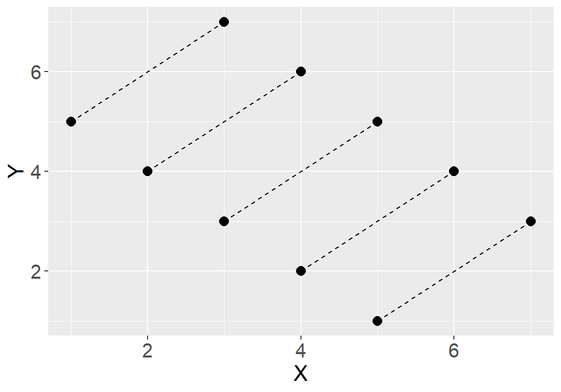
图 46.10: Artificial data: within cluster regressions

46.3.5 固定效应模型 fixed effect model

无论数据中的分层结构是否有现实意义(如果说是五种不同的民族，那就有显著的现实意义)，在回归模型中都有必要考虑这个分层结构对数据的变异的贡献 (the contribution of the clusters to the data variation)。

线性回归章节中我们使用的是五个哑变量来代表不同组别加以分析:

\[ Y_{ij} = \alpha_1 I_{i, j = 1} + \alpha_2 I_{i, j=2} + \cdots + \alpha_5 I_{i, j=5} + \beta_1X_{ij} + \varepsilon_{ ij} \]

其中 $j$ 是所属层级编号。该模型中的 $\varepsilon_{ij}$ 被认为服从均值为零，方差为 $\sigma_{\varepsilon}^2$ 的正态分布。该模型也可以简写为:

\[ Y_{ij} = \alpha_j + \beta_1X_{ij} + \epsilon_{ij} \] 一样一预案这样的模型在等级线性回归模型中被认为是固定效应模型 fixed effect model。它其实是默认给五个层级五个不同的截距，每层内部 $X,Y$ 之间的关系 (斜率) 则被认为是完全相同的 (namely the within cluster models are the same)。

本课刚开始的例子中有个数据是来自 6 所不同医院 72 名患者的收缩期血压的数据。我们现在来分析这些人中血压和年龄之间的关系。下面的散点图重现了六所医院的72名患者的血压和年龄。

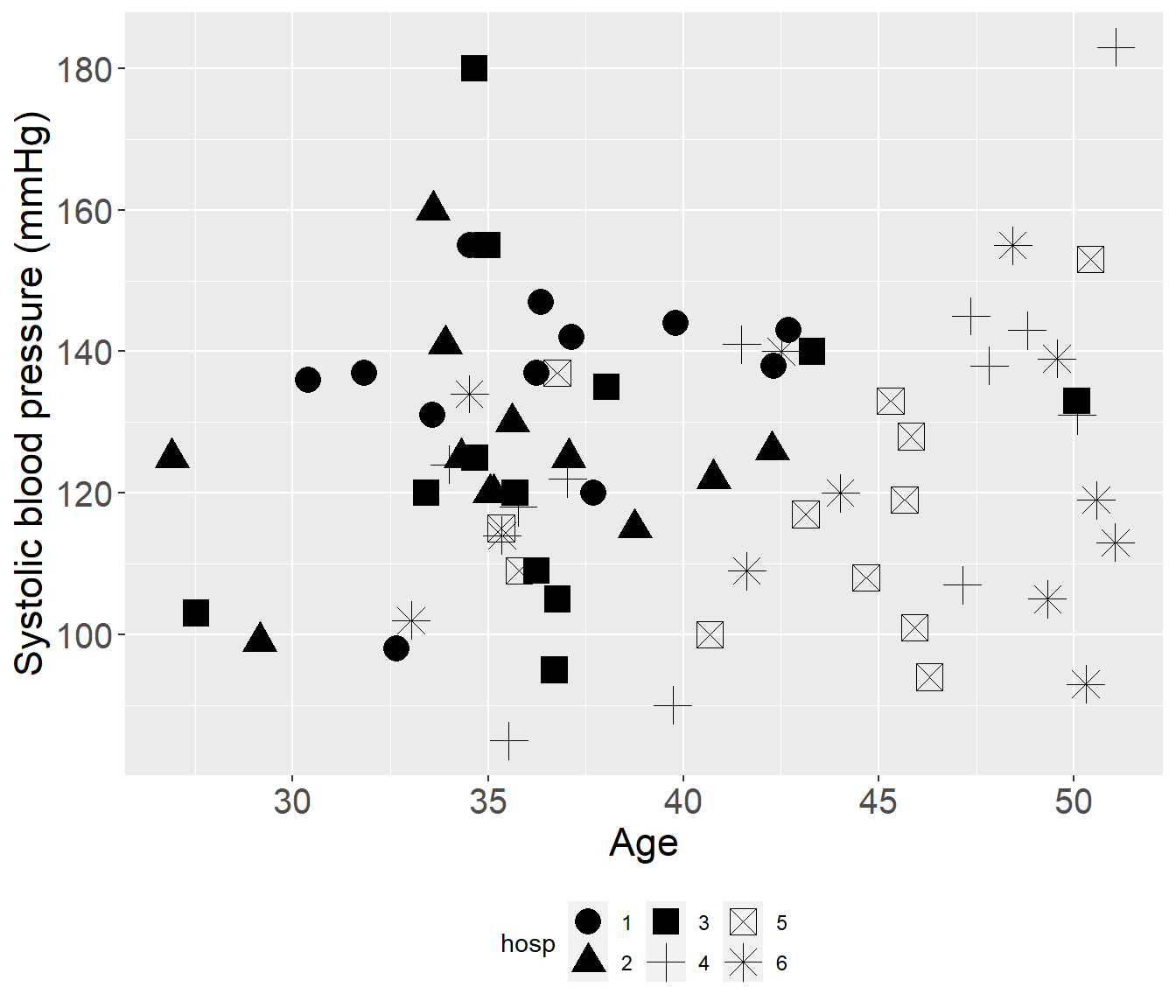
图 46.11: SBP versus age: different symbols identify the six hospitals

下面在 R 里拟合这个固定效应模型:

Bp <- read_dta("../backupfiles/bp.dta")

Bp$hosp <- as.factor(Bp$hosp)
Bp <- Bp %>%
  mutate(c_age = age - mean(age))
# 通过指定截距为零，获取每个医院的回归线的截距
Model0 <- lm(bp ~ 0 +  c_age + hosp, data = Bp) 

summary(Model0)

## 
## Call:
## lm(formula = bp ~ 0 + c_age + hosp, data = Bp)
## 
## Residuals:
##     Min      1Q  Median      3Q     Max 
## -34.780  -9.811  -0.529   7.400  55.529 
## 
## Coefficients:
##       Estimate Std. Error t value Pr(>|t|)    
## c_age   1.0022     0.4377    2.29   0.0253 *  
## hosp1 139.1542     5.7302   24.29   <2e-16 ***
## hosp2 130.2102     5.8696   22.18   <2e-16 ***
## hosp3 129.5815     5.6688   22.86   <2e-16 ***
## hosp4 124.0019     5.7033   21.74   <2e-16 ***
## hosp5 114.5886     5.7029   20.09   <2e-16 ***
## hosp6 115.7970     5.8563   19.77   <2e-16 ***
## ---
## Signif. codes:  0 '***' 0.001 '**' 0.01 '*' 0.05 '.' 0.1 ' ' 1
## 
## Residual standard error: 19.14 on 65 degrees of freedom
## Multiple R-squared:  0.9795, Adjusted R-squared:  0.9773 
## F-statistic: 444.5 on 7 and 65 DF,  p-value: < 2.2e-16

# 先生成一个新的医院变量 hops1 = 1。然后使用偏 F 检验法
# 检验控制了患者的年龄以后，这六所医院的截距是否各自不相同。
Bp$hosp1 <- Bp$hosp[1]
mod2 <- lm(bp ~ 0 +  c_age + as.numeric(hosp1), data = Bp)
anova(Model0, mod2)

## Analysis of Variance Table
## 
## Model 1: bp ~ 0 + c_age + hosp
## Model 2: bp ~ 0 + c_age + as.numeric(hosp1)
##   Res.Df   RSS Df Sum of Sq      F  Pr(>F)  
## 1     65 23802                              
## 2     70 27752 -5   -3949.7 2.1572 0.06964 .
## ---
## Signif. codes:  0 '***' 0.001 '**' 0.01 '*' 0.05 '.' 0.1 ' ' 1

偏F 检验法给出的结果$F(5, 65) = 2.16, P = 0.07$，所以说，数据其实告诉我们，调整了年龄之后，这六所医院患者中年龄和血压之间关系的回归线有不同的截距 (线性回归章节 23)。

46.4 Hierarchical例1

46.4.1 数据

High-School-and-Beyond 数据
本数据来自1982年美国国家教育统计中心 (National Center for Education Statistics, NCES) 对美国公立学校和天主教会学校的一项普查。曾经在 Hierarchical Linear Model (Raudenbush and Bryk 2002) 一书中作为范例使用。其数据的变量名和各自含义如下：

minority           indicatory of student ethinicity (1 = minority, 0 = other)
female             pupil's gender
ses                standardized socio-economic status score
mathach            measure of mathematics achievement
size               school's total number of pupils
sector             school's sector: 1 = catholic, 0 = not catholic
schoolid           school identifier

PEFR 数据
数据本身是 17 名研究对象用两种不同的测量方法测量两次每个人的最大呼气流速 (peak-expiratory-flow rate, PEFR)。最早在1986年的柳叶刀杂志发表 (Bland and Altman 1986)。两种测量法的名称分别是 “Standard Wright” 和 “Mini Wright” peak flow meter。变量名和个字含义如下：

id                 participant identifier
wp1                standard wright measure at 1st occasion
wp2                standard wright measure at 2nd occasion
wm1                mini wright measure at 1st occasion
wm2                mini wright measure at 2nd occasion

46.4.2 问题

46.4.3 将 High-School-and-Beyond 数据导入 R 中，熟悉数据结构及内容，特别要注意观察每个学校的学生特征。

library(haven)
library(epiDisplay)
library(tidyverse)
hsb_selected <- read_dta("../Datas/hsb_selected.dta")
length(unique(hsb_selected$schoolid)) ## number of school = 160

## [1] 160

## create a subset data with only the first observation of each school
hsb <- hsb_selected[!duplicated(hsb_selected$schoolid), ]

## about 44 % of the schools are Catholic schools
with(hsb, tab1(sector, graph = FALSE, decimal = 2))

## sector : 
##         Frequency Percent Cum. percent
## 0              90   56.25        56.25
## 1              70   43.75       100.00
##   Total       160  100.00       100.00

## among all the pupils, about 53% are females
with(hsb_selected, tab1(female, graph = FALSE, decimal = 2))

## female : 
##         Frequency Percent Cum. percent
## 0            3390   47.18        47.18
## 1            3795   52.82       100.00
##   Total      7185  100.00       100.00

## among all the pupils, about 27.5% are from ethnic minorities
with(hsb_selected, tab1(minority, graph = FALSE, decimal = 2))

## minority : 
##         Frequency Percent Cum. percent
## 0            5211   72.53        72.53
## 1            1974   27.47       100.00
##   Total      7185  100.00       100.00

46.4.4 为了简便起见，接下来的分析只节选数据中前五所学校 188 名学生的数学成绩，和 SES。分别计算每所学校的数学成绩,及 SES 的平均值。

hsb5 <- subset(hsb_selected, schoolid < 1320)
Mean_ses_math <- plyr::ddply(hsb5,~schoolid,summarise,mean_ses=mean(ses),mean_math=mean(mathach))
## the mean SES score ranges from -0.4255 to +0.5280
## the mean Maths score ranges from 7.636 to 16.255
Mean_ses_math

##   schoolid   mean_ses mean_math
## 1     1224 -0.4343830  9.715447
## 2     1288  0.1216000 13.510800
## 3     1296 -0.4255000  7.635958
## 4     1308  0.5280000 16.255500
## 5     1317  0.3453333 13.177688

46.4.5 先无视掉学校这一分层变量，把所有学生看作是相互独立的，拟合总体的 SES 和数学成绩的线性回归 (Total regression model)。把该总体模型的预测值提取并存储在数据库中。

## plot the scatter of mathach and ses among these 5 schools

ggplot(hsb5, aes(x = ses, y = mathach)) + geom_point() +
  theme_bw() +
  theme(axis.text = element_text(size = 15),
  axis.text.x = element_text(size = 15),
  axis.text.y = element_text(size = 15)) +
  labs(x = "SES", y = "Math achievement")  +
  xlim(-2.05, 2.05)+
  ylim(-10, 30) +
  theme(axis.title = element_text(size = 17), axis.text = element_text(size = 8))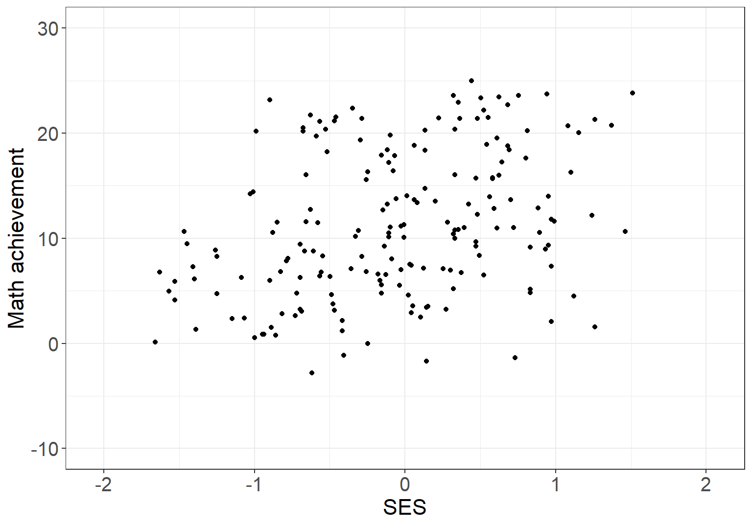

图 46.12: Scatter plot of SES and math achievements among all pupils from first 5 schools, assuming that they are all independent

Total_reg <- lm(mathach ~ ses, data = hsb5)
## the total regression model gives an estimated regression coefficient for the SES
## of each pupil equal to 3.31 (SE=0.66)
summary(Total_reg)

## 
## Call:
## lm(formula = mathach ~ ses, data = hsb5)
## 
## Residuals:
##      Min       1Q   Median       3Q      Max 
## -15.2302  -5.0832  -0.6861   5.1117  14.6851 
## 
## Coefficients:
##             Estimate Std. Error t value Pr(>|t|)    
## (Intercept)  11.4565     0.4734  24.200  < 2e-16 ***
## ses           3.3070     0.6602   5.009 1.27e-06 ***
## ---
## Signif. codes:  0 '***' 0.001 '**' 0.01 '*' 0.05 '.' 0.1 ' ' 1
## 
## Residual standard error: 6.471 on 186 degrees of freedom
## Multiple R-squared:  0.1189, Adjusted R-squared:  0.1141 
## F-statistic: 25.09 on 1 and 186 DF,  p-value: 1.267e-06

hsb5$Pred_T <- Total_reg$fitted.values # save the fitted values to the dataset

46.4.6 用各个学校 SES 和数学成绩的均值拟合一个学校间的线性回归模型 (between regression model)。

Btw_reg <- lm(mean_math ~ mean_ses, data = Mean_ses_math)
## the regression model for the school level variables (between model) gives
## an estimated regression coefficient of 7.29 (SE=1.41)
summary(Btw_reg)

## 
## Call:
## lm(formula = mean_math ~ mean_ses, data = Mean_ses_math)
## 
## Residuals:
##       1       2       3       4       5 
##  1.0201  0.7621 -1.1241  0.5440 -1.2021 
## 
## Coefficients:
##             Estimate Std. Error t value Pr(>|t|)    
## (Intercept)  11.8622     0.5566  21.310 0.000226 ***
## mean_ses      7.2904     1.4070   5.181 0.013956 *  
## ---
## Signif. codes:  0 '***' 0.001 '**' 0.01 '*' 0.05 '.' 0.1 ' ' 1
## 
## Residual standard error: 1.242 on 3 degrees of freedom
## Multiple R-squared:  0.8995, Adjusted R-squared:  0.866 
## F-statistic: 26.85 on 1 and 3 DF,  p-value: 0.01396

Mean_ses_math$Pred_B <- Btw_reg$fitted.values # save the fitted values to the dataset

46.4.7 分别对每个学校内的学生进行 SES 和数学成绩拟合线性回归模型。

Within_schl1 <- lm(mathach ~ ses, data = hsb5[hsb5$schoolid == 1224,])
Within_schl2 <- lm(mathach ~ ses, data = hsb5[hsb5$schoolid == 1288,])
Within_schl3 <- lm(mathach ~ ses, data = hsb5[hsb5$schoolid == 1296,])
Within_schl4 <- lm(mathach ~ ses, data = hsb5[hsb5$schoolid == 1308,])
Within_schl5 <- lm(mathach ~ ses, data = hsb5[hsb5$schoolid == 1317,])
# the within school regressions gives estimated slopes which have a mean of 1.65
# and which ranges between 0.126 and 3.255
summary(c(Within_schl1$coefficients[2], Within_schl2$coefficients[2],
      Within_schl3$coefficients[2], Within_schl4$coefficients[2],
      Within_schl5$coefficients[2]))

##    Min. 1st Qu.  Median    Mean 3rd Qu.    Max. 
##   0.126   1.076   1.274   1.648   2.509   3.255

# the SEs ranging between 1.21 and 3.00
summary(c(summary(Within_schl1)$coefficients[4],
          summary(Within_schl2)$coefficients[4],
          summary(Within_schl3)$coefficients[4],
          summary(Within_schl4)$coefficients[4],
          summary(Within_schl5)$coefficients[4]))

##    Min. 1st Qu.  Median    Mean 3rd Qu.    Max. 
##   1.209   1.436   1.765   1.899   2.080   3.003

hsb5$Pred_W <- c(Within_schl1$fitted.values, Within_schl2$fitted.values,
      Within_schl3$fitted.values, Within_schl4$fitted.values,
      Within_schl5$fitted.values) ## save the predicted value into the dataset

46.4.8 比较三种模型计算的数学成绩的拟合值，他们一致？还是有所不同？为什么会有不同？

总体模型 (Total regression model) 实际上无视了学生的性别，种族等可能带来的混杂效果；
学校间模型(Between model) 估计的实际上是SES均值每增加一个单位，与之对应的数学平均成绩的改变量，这个模型绝对不可用与评估个人的SES 与数学成绩之间的关系；
学校内模型 (Within model) 拟合的 SES 与数学成绩之间的关系变得十分地不精确 (SEs are fairly large)，变化幅度也很大。

46.4.9 把三种模型的数学成绩拟合值散点图绘制在同一张图内。

Mean <- Mean_ses_math[, 1:3]
names(Mean) <- c("schoolid", "ses", "Pred_W")


ggplot(hsb5, aes(x = ses, y = Pred_W, group = schoolid)) +
  geom_line(linetype = 2, size = 1) +
  geom_abline(intercept = Total_reg$coefficients[1], slope = Total_reg$coefficients[2],
               colour = "dark blue") +
  geom_abline(intercept = Btw_reg$coefficients[1], slope = Btw_reg$coefficients[2],
               colour = "red") +
  geom_point(data = Mean, shape = 17, size = 4, colour = "Red") +
  theme_bw() +
  theme(axis.text = element_text(size = 15),
  axis.text.x = element_text(size = 15),
  axis.text.y = element_text(size = 15)) +
  labs(x = "SES", y = "Fitted regression lines (Maths achievement)")  +
  xlim(-2.05, 2.05)+
  ylim(5, 20) +
  theme(axis.title = element_text(size = 17), axis.text = element_text(size = 8)) + 
  theme(plot.caption = element_text(size = 12,
  hjust = 0)) + labs(caption = "Black dash line: Within regression model;
Blue solid line: Total regression model;
Red solid line: Between regression model;
Red triangle: School mean values")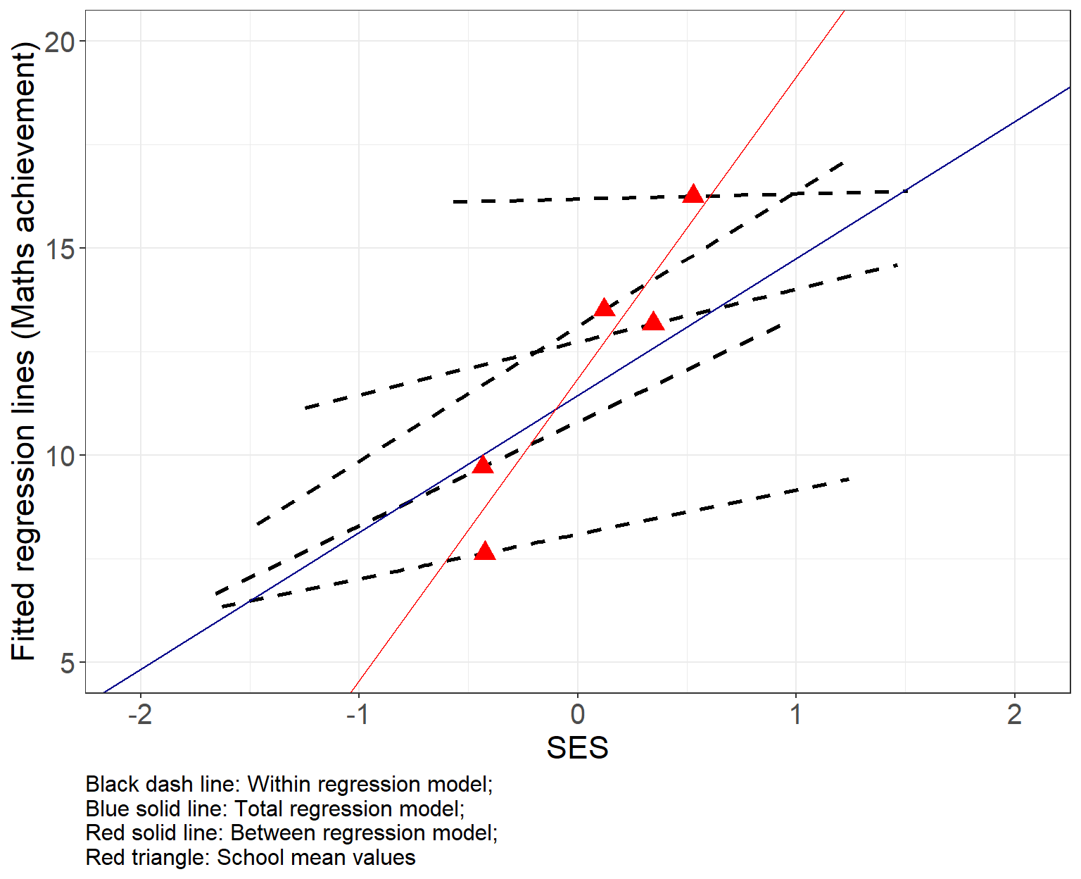

图 46.13: High-school-and-beyond data: Predicted values by Total, Between, and Within regression models

46.4.10 用这 5 个学校的数据拟合一个固定效应线性回归模型

Fixed_reg <- lm(mathach ~ ses + factor(schoolid), data = hsb5)

## Fitting a fixed effect model to these data is equivalent to forcing
## a common slope onto the five within regression models. It gives an
## estimated slope of 1.789 (SE=0.76), close to their average of 1.64799.
## Note that controlling for female, minority, and sector but not for
## schoolid leads to roughly the same estimate (slope = 1.68, SE=0.75)

summary(Fixed_reg)

## 
## Call:
## lm(formula = mathach ~ ses + factor(schoolid), data = hsb5)
## 
## Residuals:
##      Min       1Q   Median       3Q      Max 
## -13.9759  -4.1968  -0.7519   5.2209  16.3813 
## 
## Coefficients:
##                      Estimate Std. Error t value Pr(>|t|)    
## (Intercept)           10.4925     0.9676  10.844  < 2e-16 ***
## ses                    1.7890     0.7594   2.356  0.01955 *  
## factor(schoolid)1288   2.8007     1.6004   1.750  0.08180 .  
## factor(schoolid)1296  -2.0954     1.2797  -1.637  0.10328    
## factor(schoolid)1308   4.8184     1.8183   2.650  0.00876 ** 
## factor(schoolid)1317   2.0674     1.4101   1.466  0.14433    
## ---
## Signif. codes:  0 '***' 0.001 '**' 0.01 '*' 0.05 '.' 0.1 ' ' 1
## 
## Residual standard error: 6.236 on 182 degrees of freedom
## Multiple R-squared:  0.1992, Adjusted R-squared:  0.1772 
## F-statistic: 9.054 on 5 and 182 DF,  p-value: 1.051e-07

summary(lm(mathach ~ ses + female + minority + sector, data = hsb5))

## 
## Call:
## lm(formula = mathach ~ ses + female + minority + sector, data = hsb5)
## 
## Residuals:
##      Min       1Q   Median       3Q      Max 
## -13.0913  -4.1733  -0.4631   4.5081  15.3320 
## 
## Coefficients:
##             Estimate Std. Error t value Pr(>|t|)    
## (Intercept)  12.5454     0.8603  14.583  < 2e-16 ***
## ses           1.6805     0.7449   2.256 0.025248 *  
## female       -1.5486     0.9486  -1.633 0.104278    
## minority     -3.1963     0.9545  -3.349 0.000986 ***
## sector        3.9812     1.1194   3.557 0.000478 ***
## ---
## Signif. codes:  0 '***' 0.001 '**' 0.01 '*' 0.05 '.' 0.1 ' ' 1
## 
## Residual standard error: 6.17 on 183 degrees of freedom
## Multiple R-squared:  0.2119, Adjusted R-squared:  0.1947 
## F-statistic:  12.3 on 4 and 183 DF,  p-value: 7.026e-09

46.4.11 PEFR 数据

pefr <- read_dta("../Datas/pefr.dta")
# the data are in wide format
pefr

## # A tibble: 17 × 5
##       id   wp1   wp2   wm1   wm2
##    <dbl> <dbl> <dbl> <dbl> <dbl>
##  1     1   494   490   512   525
##  2     2   395   397   430   415
##  3     3   516   512   520   508
##  4     4   434   401   428   444
##  5     5   476   470   500   500
##  6     6   557   611   600   625
##  7     7   413   415   364   460
##  8     8   442   431   380   390
##  9     9   650   638   658   642
## 10    10   433   429   445   432
## 11    11   417   420   432   420
## 12    12   656   633   626   605
## 13    13   267   275   260   227
## 14    14   478   492   477   467
## 15    15   178   165   259   268
## 16    16   423   372   350   370
## 17    17   427   421   451   443

# transform data into long format
pefr_long <- pefr %>%
  gather(key, value, -id) %>%
  separate(key, into = c("measurement", "occasion"), sep = 2) %>%
  arrange(id, occasion) %>%
  spread(measurement, value)
pefr_long

## # A tibble: 34 × 4
##       id occasion    wm    wp
##    <dbl> <chr>    <dbl> <dbl>
##  1     1 1          512   494
##  2     1 2          525   490
##  3     2 1          430   395
##  4     2 2          415   397
##  5     3 1          520   516
##  6     3 2          508   512
##  7     4 1          428   434
##  8     4 2          444   401
##  9     5 1          500   476
## 10     5 2          500   470
## # ℹ 24 more rows

## figure shows slightly closer agreement between the repeated measures of standard Wright,
## than between those of Mini Wright

ggplot(pefr_long, aes(x = id, y = wp, fill = occasion)) +
  geom_point(size = 4, shape = 21) +
  geom_hline(yintercept = mean(pefr_long$wp), colour = "red") +
  theme_bw() +
  scale_x_continuous(breaks = 1:17)+
  theme(axis.text = element_text(size = 15),
  axis.text.x = element_text(size = 15),
  axis.text.y = element_text(size = 15)) +
  labs(x = "Subject ID", y = "W Measurements")  +
  theme(axis.title = element_text(size = 17), axis.text = element_text(size = 8))+ 
  theme(legend.text = element_text(size = 19), 
  legend.title = element_text(size = 19))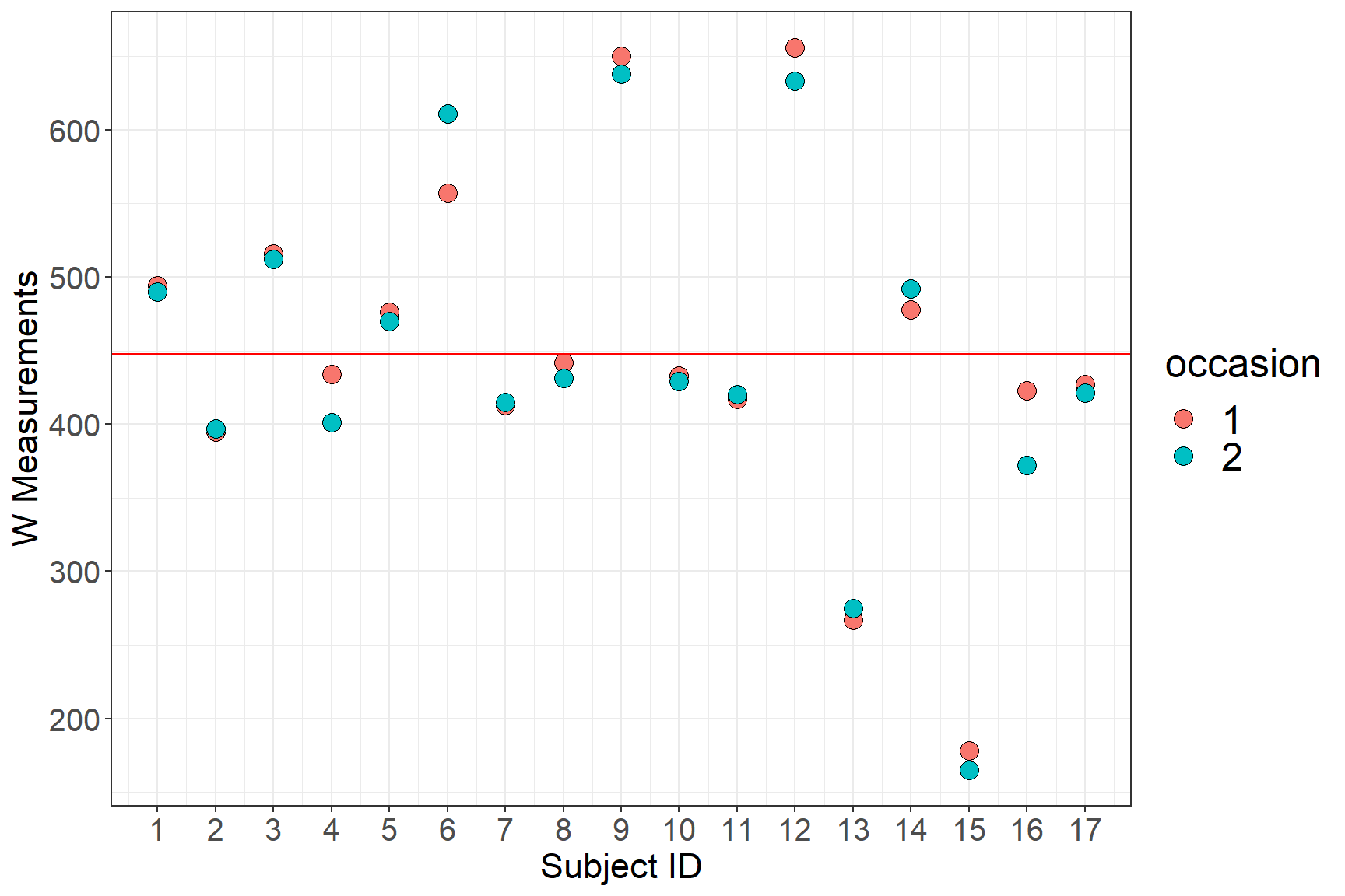

图 46.14: Two recordings of PEFR taken with the standard Wright meter

46.4.12 求每个患者的 `wp` 两次测量平均值

# the means range from 171.5 to 644.5
pefr_long %>% 
  group_by(id) %>% 
  summarise(mean_wp = mean(wp))

## # A tibble: 17 × 2
##       id mean_wp
##    <dbl>   <dbl>
##  1     1    492 
##  2     2    396 
##  3     3    514 
##  4     4    418.
##  5     5    473 
##  6     6    584 
##  7     7    414 
##  8     8    436.
##  9     9    644 
## 10    10    431 
## 11    11    418.
## 12    12    644.
## 13    13    271 
## 14    14    485 
## 15    15    172.
## 16    16    398.
## 17    17    424

46.4.13 在 R 里先用 ANOVA 分析个人的 `wp` 变异。再用 `lme4::lmer` 拟合用 `id` 作随机效应的混合效应模型。确认后者报告的`Std.Dev for id effect` 其实可以用ANOVA 结果的$\sqrt{\frac{\text{MMS-MSE}}{n}}$ (n 是每个个体重复测量值的个数)。

with(pefr_long, anova(lm(wp~factor(id))))

## Analysis of Variance Table
## 
## Response: wp
##            Df Sum Sq Mean Sq F value    Pr(>F)    
## factor(id) 16 441599 27599.9   117.8 3.145e-14 ***
## Residuals  17   3983   234.3                      
## ---
## Signif. codes:  0 '***' 0.001 '**' 0.01 '*' 0.05 '.' 0.1 ' ' 1

#library(lme4)
( fit <- lme4::lmer(wp ~ (1|id), data=pefr_long) )

## Linear mixed model fit by REML ['lmerMod']
## Formula: wp ~ (1 | id)
##    Data: pefr_long
## REML criterion at convergence: 353.5472
## Random effects:
##  Groups   Name        Std.Dev.
##  id       (Intercept) 116.97  
##  Residual              15.31  
## Number of obs: 34, groups:  id, 17
## Fixed Effects:
## (Intercept)  
##       447.9

sqrt((27600 - 234)/2)

## [1] 116.9744

46.4.14 拟合结果变量为 `wp`，解释变量为 `id` 的简单线性回归模型。用数学表达式描述这个模型。

Reg <- lm(wp ~ factor(id), data = pefr_long)

# The fixed effect regression model leads to the same ANOVA
# table. To the same estimate of the residual SD = (15.307)
# However, it does not give an estimate of the "SD of id effect"
# Instead it gives estimates of mean PEFR for participant number 1
# = 492 and estimates of the difference in means from him/her
# for all the other 16 pariticipants
anova(Reg)

## Analysis of Variance Table
## 
## Response: wp
##            Df Sum Sq Mean Sq F value    Pr(>F)    
## factor(id) 16 441599 27599.9   117.8 3.145e-14 ***
## Residuals  17   3983   234.3                      
## ---
## Signif. codes:  0 '***' 0.001 '**' 0.01 '*' 0.05 '.' 0.1 ' ' 1

summary(Reg)

## 
## Call:
## lm(formula = wp ~ factor(id), data = pefr_long)
## 
## Residuals:
##    Min     1Q Median     3Q    Max 
## -27.00  -3.75   0.00   3.75  27.00 
## 
## Coefficients:
##              Estimate Std. Error t value Pr(>|t|)    
## (Intercept)    492.00      10.82  45.457  < 2e-16 ***
## factor(id)2    -96.00      15.31  -6.272 8.44e-06 ***
## factor(id)3     22.00      15.31   1.437 0.168789    
## factor(id)4    -74.50      15.31  -4.867 0.000145 ***
## factor(id)5    -19.00      15.31  -1.241 0.231355    
## factor(id)6     92.00      15.31   6.010 1.40e-05 ***
## factor(id)7    -78.00      15.31  -5.096 8.97e-05 ***
## factor(id)8    -55.50      15.31  -3.626 0.002088 ** 
## factor(id)9    152.00      15.31   9.930 1.72e-08 ***
## factor(id)10   -61.00      15.31  -3.985 0.000957 ***
## factor(id)11   -73.50      15.31  -4.802 0.000166 ***
## factor(id)12   152.50      15.31   9.963 1.63e-08 ***
## factor(id)13  -221.00      15.31 -14.438 5.67e-11 ***
## factor(id)14    -7.00      15.31  -0.457 0.653233    
## factor(id)15  -320.50      15.31 -20.939 1.41e-13 ***
## factor(id)16   -94.50      15.31  -6.174 1.02e-05 ***
## factor(id)17   -68.00      15.31  -4.443 0.000357 ***
## ---
## Signif. codes:  0 '***' 0.001 '**' 0.01 '*' 0.05 '.' 0.1 ' ' 1
## 
## Residual standard error: 15.31 on 17 degrees of freedom
## Multiple R-squared:  0.9911, Adjusted R-squared:  0.9826 
## F-statistic: 117.8 on 16 and 17 DF,  p-value: 3.145e-14

上面的模型用数学表达式来描述就是：

\[ \begin{aligned} Y_{ij} & = \alpha_1 + \delta_i + \varepsilon_{ij} \\ \text{Where } \delta_j & = \alpha_j - \alpha_1 \\ \text{and } \delta_1 & = 0 \end{aligned} \]

46.4.15 将 `wp` 中心化之后，重新拟合相同的模型，把截距去除掉。写下这个模型的数学表达式。

Reg1 <- lm((wp - mean(wp)) ~ 0 + factor(id), data = pefr_long)

# it leads to the same ANOVA table again, same residual SD
anova(Reg1)

## Analysis of Variance Table
## 
## Response: (wp - mean(wp))
##            Df Sum Sq Mean Sq F value    Pr(>F)    
## factor(id) 17 441599 25976.4  110.87 4.535e-14 ***
## Residuals  17   3983   234.3                      
## ---
## Signif. codes:  0 '***' 0.001 '**' 0.01 '*' 0.05 '.' 0.1 ' ' 1

summary(Reg1)

## 
## Call:
## lm(formula = (wp - mean(wp)) ~ 0 + factor(id), data = pefr_long)
## 
## Residuals:
##    Min     1Q Median     3Q    Max 
## -27.00  -3.75   0.00   3.75  27.00 
## 
## Coefficients:
##              Estimate Std. Error t value Pr(>|t|)    
## factor(id)1     44.12      10.82   4.076 0.000786 ***
## factor(id)2    -51.88      10.82  -4.794 0.000169 ***
## factor(id)3     66.12      10.82   6.109 1.16e-05 ***
## factor(id)4    -30.38      10.82  -2.807 0.012123 *  
## factor(id)5     25.12      10.82   2.321 0.032995 *  
## factor(id)6    136.12      10.82  12.576 4.89e-10 ***
## factor(id)7    -33.88      10.82  -3.130 0.006093 ** 
## factor(id)8    -11.38      10.82  -1.052 0.307685    
## factor(id)9    196.12      10.82  18.120 1.49e-12 ***
## factor(id)10   -16.88      10.82  -1.560 0.137230    
## factor(id)11   -29.38      10.82  -2.715 0.014716 *  
## factor(id)12   196.62      10.82  18.166 1.43e-12 ***
## factor(id)13  -176.88      10.82 -16.343 7.89e-12 ***
## factor(id)14    37.12      10.82   3.429 0.003198 ** 
## factor(id)15  -276.38      10.82 -25.536 5.34e-15 ***
## factor(id)16   -50.38      10.82  -4.655 0.000227 ***
## factor(id)17   -23.88      10.82  -2.207 0.041389 *  
## ---
## Signif. codes:  0 '***' 0.001 '**' 0.01 '*' 0.05 '.' 0.1 ' ' 1
## 
## Residual standard error: 15.31 on 17 degrees of freedom
## Multiple R-squared:  0.9911, Adjusted R-squared:  0.9821 
## F-statistic: 110.9 on 17 and 17 DF,  p-value: 4.535e-14

上面的模型用数学表达式来描述就是：

\[ \begin{aligned} Y_{ij} - \mu & = \gamma_j + \varepsilon_{ij} \\ Y_{ij} & = \mu + \gamma_j + \varepsilon_{ij} \\ \text{Where } \mu & \text{ is the overall mean} \\ \text{and } \sum_{j=1}^J\gamma_j & = 0\\ \end{aligned} \]

46.4.16 计算这些回归系数 (其实是不同群之间的随机截距) 的均值和标准差。

# the individual level intercepts have mean zero and SD = 117.47, larger than the estimated
# Std.Dev for id effect.
Reg1$coefficients

##  factor(id)1  factor(id)2  factor(id)3  factor(id)4  factor(id)5  factor(id)6 
##     44.11765    -51.88235     66.11765    -30.38235     25.11765    136.11765 
##  factor(id)7  factor(id)8  factor(id)9 factor(id)10 factor(id)11 factor(id)12 
##    -33.88235    -11.38235    196.11765    -16.88235    -29.38235    196.61765 
## factor(id)13 factor(id)14 factor(id)15 factor(id)16 factor(id)17 
##   -176.88235     37.11765   -276.38235    -50.38235    -23.88235

mean(Reg1$coefficients)

## [1] 7.62513e-15

sd(Reg1$coefficients)

## [1] 117.4732

Reference

Bland, J Martin, and DouglasG Altman. 1986. “Statistical Methods for Assessing Agreement Between Two Methods of Clinical Measurement.” The Lancet 327 (8476): 307–10.

Raudenbush, Stephen W, and Anthony S Bryk. 2002. Hierarchical Linear Models: Applications and Data Analysis Methods. Vol. 1. Sage.

Robinson, W. S. 1950. “Ecological Correlations and the Behavior of Individuals.” American Sociological Review 15 (3): 351–57. http://www.jstor.org/stable/2087176.

Snijders, Tom, and Roel Bosker. 1999. “Multilevel Analysis: An Introduction to Basic and Applied Multilevel Analysis.” London: Sage.

Cluster \((j)\)	id \((i)\)	\(X\)	\(Y\)	\(\bar{X}\)	\(\bar{Y}\)
1	1	1	5	2	6
1	2	3	7	2	6
2	1	2	4	3	5
2	2	4	6	3	5
3	1	3	3	4	4
3	2	5	5	4	4
4	1	4	2	5	3
4	2	6	4	5	3
5	1	5	1	6	2
5	2	7	3	6	2

R语言与医学统计

第 46 章相互依赖数据及简单的应对方案

46.1 相互依赖的数据

46.2 数据有依赖性导致的结果

46.3 边际模型和条件模型 marginal and conditional models

46.3.1 标记法 notation

46.3.2 合并每个阶层

46.3.3 生物学悖论 ecological fallacy

46.3.4 分解层级数据

46.3.5 固定效应模型 fixed effect model

46.4 Hierarchical例1

46.4.1 数据

46.4.2 问题

46.4.3 将 High-School-and-Beyond 数据导入 R 中，熟悉数据结构及内容，特别要注意观察每个学校的学生特征。

46.4.4 为了简便起见，接下来的分析只节选数据中前五所学校 188 名学生的数学成绩，和 SES。分别计算每所学校的数学成绩,及 SES 的平均值。

46.4.5 先无视掉学校这一分层变量，把所有学生看作是相互独立的，拟合总体的 SES 和数学成绩的线性回归 (Total regression model)。把该总体模型的预测值提取并存储在数据库中。

46.4.6 用各个学校 SES 和数学成绩的均值拟合一个学校间的线性回归模型 (between regression model)。

46.4.7 分别对每个学校内的学生进行 SES 和数学成绩拟合线性回归模型。

46.4.8 比较三种模型计算的数学成绩的拟合值，他们一致？还是有所不同？为什么会有不同？

46.4.9 把三种模型的数学成绩拟合值散点图绘制在同一张图内。

46.4.10 用这 5 个学校的数据拟合一个固定效应线性回归模型

46.4.11 PEFR 数据

46.4.12 求每个患者的 `wp` 两次测量平均值

46.4.13 在 R 里先用 ANOVA 分析个人的 `wp` 变异。再用 `lme4::lmer` 拟合用 `id` 作随机效应的混合效应模型。确认后者报告的`Std.Dev for id effect` 其实可以用ANOVA 结果的\(\sqrt{\frac{\text{MMS-MSE}}{n}}\) (n 是每个个体重复测量值的个数)。

46.4.14 拟合结果变量为 `wp`，解释变量为 `id` 的简单线性回归模型。用数学表达式描述这个模型。

46.4.15 将 `wp` 中心化之后，重新拟合相同的模型，把截距去除掉。写下这个模型的数学表达式。

46.4.16 计算这些回归系数 (其实是不同群之间的随机截距) 的均值和标准差。

Reference

Cluster (j)	id (i)	X	Y	X	Y
1	1	1	5	2	6
1	2	3	7	2	6
2	1	2	4	3	5
2	2	4	6	3	5
3	1	3	3	4	4
3	2	5	5	4	4
4	1	4	2	5	3
4	2	6	4	5	3
5	1	5	1	6	2
5	2	7	3	6	2

Cluster \((j)\)	id \((i)\)	\(X\)	\(Y\)	\(\bar{X}\)	\(\bar{Y}\)
1	1	1	5	2	6
1	2	3	7	2	6
2	1	2	4	3	5
2	2	4	6	3	5
3	1	3	3	4	4
3	2	5	5	4	4
4	1	4	2	5	3
4	2	6	4	5	3
5	1	5	1	6	2
5	2	7	3	6	2

Cluster (j)	id (i)	X	Y	X	Y
1	1	1	5	2	6
1	2	3	7	2	6
2	1	2	4	3	5
2	2	4	6	3	5
3	1	3	3	4	4
3	2	5	5	4	4
4	1	4	2	5	3
4	2	6	4	5	3
5	1	5	1	6	2
5	2	7	3	6	2

Cluster \((j)\)	id \((i)\)	\(X\)	\(Y\)	\(\bar{X}\)	\(\bar{Y}\)
1	1	1	5	2	6
1	2	3	7	2	6
2	1	2	4	3	5
2	2	4	6	3	5
3	1	3	3	4	4
3	2	5	5	4	4
4	1	4	2	5	3
4	2	6	4	5	3
5	1	5	1	6	2
5	2	7	3	6	2

第 46 章 相互依赖数据及简单的应对方案

46.1 相互依赖的数据

46.2 数据有依赖性导致的结果

46.3 边际模型和条件模型 marginal and conditional models

46.3.1 标记法 notation

46.3.2 合并每个阶层

46.3.3 生物学悖论 ecological fallacy

46.3.4 分解层级数据

46.3.5 固定效应模型 fixed effect model

46.4 Hierarchical例1

46.4.1 数据

46.4.2 问题

46.4.3 将 High-School-and-Beyond 数据导入 R 中，熟悉数据结构及内容，特别要注意观察每个学校的学生特征。

46.4.4 为了简便起见，接下来的分析只节选数据中前五所学校 188 名学生的数学成绩，和 SES。分别计算每所学校的数学成绩,及 SES 的平均值。

46.4.5 先无视掉学校这一分层变量，把所有学生看作是相互独立的，拟合总体的 SES 和数学成绩的线性回归 (Total regression model)。把该总体模型的预测值提取并存储在数据库中。

46.4.6 用各个学校 SES 和数学成绩的均值拟合一个学校间的线性回归模型 (between regression model)。

46.4.7 分别对每个学校内的学生进行 SES 和数学成绩拟合线性回归模型。

46.4.8 比较三种模型计算的数学成绩的拟合值，他们一致？还是有所不同？为什么会有不同？

46.4.9 把三种模型的数学成绩拟合值散点图绘制在同一张图内。

46.4.10 用这 5 个学校的数据拟合一个固定效应线性回归模型

46.4.11 PEFR 数据

46.4.12 求每个患者的 wp 两次测量平均值

46.4.13 在 R 里先用 ANOVA 分析个人的 wp 变异。再用 lme4::lmer 拟合用 id 作随机效应的混合效应模型。确认后者报告的Std.Dev for id effect 其实可以用ANOVA 结果的\(\sqrt{\frac{\text{MMS-MSE}}{n}}\) (n 是每个个体重复测量值的个数)。

46.4.14 拟合结果变量为 wp，解释变量为 id 的简单线性回归模型。用数学表达式描述这个模型。

46.4.15 将 wp 中心化之后，重新拟合相同的模型，把截距去除掉。写下这个模型的数学表达式。

46.4.16 计算这些回归系数 (其实是不同群之间的随机截距) 的均值和标准差。

Reference

第 46 章相互依赖数据及简单的应对方案

46.4.12 求每个患者的 `wp` 两次测量平均值

46.4.13 在 R 里先用 ANOVA 分析个人的 `wp` 变异。再用 `lme4::lmer` 拟合用 `id` 作随机效应的混合效应模型。确认后者报告的`Std.Dev for id effect` 其实可以用ANOVA 结果的\(\sqrt{\frac{\text{MMS-MSE}}{n}}\) (n 是每个个体重复测量值的个数)。

46.4.14 拟合结果变量为 `wp`，解释变量为 `id` 的简单线性回归模型。用数学表达式描述这个模型。

46.4.15 将 `wp` 中心化之后，重新拟合相同的模型，把截距去除掉。写下这个模型的数学表达式。

Cluster (j)	id (i)	X	Y	X	Y
1	1	1	5	2	6
1	2	3	7	2	6
2	1	2	4	3	5
2	2	4	6	3	5
3	1	3	3	4	4
3	2	5	5	4	4
4	1	4	2	5	3
4	2	6	4	5	3
5	1	5	1	6	2
5	2	7	3	6	2

Cluster \((j)\)	id \((i)\)	\(X\)	\(Y\)	\(\bar{X}\)	\(\bar{Y}\)
1	1	1	5	2	6
1	2	3	7	2	6
2	1	2	4	3	5
2	2	4	6	3	5
3	1	3	3	4	4
3	2	5	5	4	4
4	1	4	2	5	3
4	2	6	4	5	3
5	1	5	1	6	2
5	2	7	3	6	2