第 38 章率的广义线性回归

38.1 医学中的率

前章介绍的事件发生次数，使用的是泊松回归。本章介绍同样利用泊松回归，对事件发生率类型数据的泊松回归模型。常见的率的数据例如：

肺癌发病率
工厂职工的死亡率
术后后遗症的发生率

下列数据来自英国医生调查 (British doctors study)，研究的是男性医生中吸烟与否和冠心病死亡之间的关系。最后一列是每组观测对象被追踪的人年 (person-year)。

   agegrp     smokes deaths  pyrs
1   35-44     Smoker     32 52407
2   45-54     Smoker    104 43248
3   55-64     Smoker    206 28612
4   65-74     Smoker    186 12663
5     75+     Smoker    102  5317
6   35-44 Non-smoker      2 18790
7   45-54 Non-smoker     12 10673
8  55-64  Non-smoker     28  5710
9   65-74 Non-smoker     28  2585
10    75+ Non-smoker     31  1462

这是一个已经被整理过的数据，我们没有办法从这样的数据还原到每个观察对象的个人水平数据。冠心病的粗死亡率 (crude death rate) 可以被计算如下表 (忽略年龄分组)，此时默认的前提是死亡事件在追踪的过程中发生的概率不发生改变。

表 38.1: Death rates due to CHD in smokers and non-smokers, collapsed over age group
Group	Person-years of follow-up	CHD deaths	Death Rate per 1000 person-years	Rate Ratios
Non-smokers	39220	101	2.58	1.00
Smokers	142247	630	4.43	1.72

38.2 泊松过程

设 \(Y\) 是代表某段时间 \(t\) 内事件发生次数 (死亡) 的随机变量。如果可以假设：

每次事件的发生，是互相独立的，即在没有重叠的时间线上，每个事件的发生是随机的。
在一个无限小的时间段 \(\delta t\) 内，事件发生的概率是 \(\lambda\times\delta t\)，其中 \(\delta t \rightarrow 0\)。

那么根据泊松分布 (Section 6) 的定义，在这个时间段内，随机变量 \(Y\) 事件发生次数服从泊松分布：

\[ \begin{aligned} Y & \sim \text{Po}(\mu) \\ \text{Where } \mu & = \lambda t, \text{ and } \lambda \text{ is the Rate} \end{aligned} \]

所以，从泊松过程可以看到，我们关心的参数是事件发生率 \(\lambda\)。

38.3 率的模型

既然关心的参数只是发生率，且我们已知泊松分布是指数分布的家族成员，可以用广义线性模型的概念来建模。

因变量分布，distribution of dependent variable \[Y_i \sim \text{Po}(\mu_i), \text{ where } \mu_i = \lambda_i t_i\]
线性预测方程，linear predictor \[\eta_i = \alpha + \beta_1 x_{i1} + \cdots + \beta_p x_{ip}\]
标准链接方程，canonical link function \[\text{log}(\lambda_i) = \text{log}(\frac{\mu_i}{t_i})\]

所以，将率的模型整理一下，就变成了

\[ \begin{aligned} \text{log}(\mu_i) - \text{log}(t_i) & = \alpha + \beta_1 x_{i1} + \cdots + \beta_p x_{ip} \\ \text{log}(\mu_i) & = \text{log}(t_i) + \alpha + \beta_1 x_{i1} + \cdots + \beta_p x_{ip} \end{aligned} \]

你可以看到，时间项的对数部分\(\text{log}(t_i)\) 其实是被移到线性预测方程的右边跟参数放在一起的，只是**它的回归系数被强制为\(1\)* *。这个时间项被叫做 补偿项 (offset)。这样我们就成功地拟合了用于求事件发生率的一个泊松回归模型。在R 里，你可以用glm() 命令的offset = 选项功能，也可以把offset(log(Person-year)) 作为线性预测方程的一部分把时间项取对数以后放进模型里面。

38.4 率的 GLM

所以我们一起来把率的 GLM 正式定义一下，它包含三个部分：

可被认为互相独立的因变量观测值的分布服从泊松分布\[Y_i \sim \text{Po}(\mu_i)\]
其中\(E(Y_i) = \mu_i = \lambda_i t_i\)，\(t_i\) 是第\(i\) 个观察对象(或者观察组) 的追踪人年(person-time)。
线性预测方程 \[\eta_i = \text{log}(t_i) + \alpha + \beta_1 x_{i1} + \cdots + \beta_p x_{ip}\]
链接方程是均值的对数方程 \[\text{log}(\mu_i) = \eta_i\]

和分组型二项分布数据相似，如果泊松 GLM 拟合的数据也是分组型数据，如本章开头的英国医生队列数据。那么模型偏差值 (deviance) 可以用来衡量模型拟合的好坏。在零假设条件下，模型偏差值服从自由度为\(n-p\) 的卡方分布(这里的\(n\) 是分组型数据中的“组的数量”，也就是饱和模型中参数的数量，\(p\)是拟合的线性预测方程中参数的数量)。

38.5 分析实例 Example: British doctors study

数据是本章开头使用的英国医生队列

   agegrp     smokes deaths  pyrs
1   35-44     Smoker     32 52407
2   45-54     Smoker    104 43248
3   55-64     Smoker    206 28612
4   65-74     Smoker    186 12663
5     75+     Smoker    102  5317
6   35-44 Non-smoker      2 18790
7   45-54 Non-smoker     12 10673
8  55-64  Non-smoker     28  5710
9   65-74 Non-smoker     28  2585
10    75+ Non-smoker     31  1462

每组的死亡人数用 \(y_i, i=1,\cdots,10\) 标记；
每组追踪的人年用 \(t_i\) 标记；
\(x_{i1} = 0\) 时对象是吸烟者，\(x_{i1} = 1\) 时对象是非吸烟者；
\(x_{i2}, x_{i3}, x_{i4}, x_{i5}\) 作为5个年龄组的哑变量。

分析目的是：

调查吸烟与冠心病死亡率的关系 (不调整年龄)；
调查吸烟与冠心病死亡率的年龄调整后关系；
调查年龄是否对吸烟与冠心病死亡率的关系起到交互作用。

38.5.1 模型 1: 吸烟

第一个模型可以用下面的数学表达式：

\[ \text{log}(\mu_i) = \text{log}(t_i) + \alpha + \beta_1 x_{i1} \]

在 R 里面用下面的代码来拟合这个模型，仔细阅读输出的结果：

# the following 2 models are equivalent
Model1 <- glm(deaths ~ smokes + offset(log(pyrs)), family = poisson(link = "log"), data = BritishD)
Model1 <- glm(deaths ~ smokes, offset = log(pyrs), family = poisson(link = "log"), data = BritishD)
summary(Model1); jtools::summ(Model1, digits = 6, confint = TRUE, exp = TRUE)


Call:
glm(formula = deaths ~ smokes, family = poisson(link = "log"), 
    data = BritishD, offset = log(pyrs))

Coefficients:
             Estimate Std. Error z value Pr(>|z|)    
(Intercept)   -5.9618     0.0995 -59.916  < 2e-16 ***
smokesSmoker   0.5422     0.1072   5.059 4.22e-07 ***
---
Signif. codes:  0 '***' 0.001 '**' 0.01 '*' 0.05 '.' 0.1 ' ' 1

(Dispersion parameter for poisson family taken to be 1)

    Null deviance: 935.07  on 9  degrees of freedom
Residual deviance: 905.98  on 8  degrees of freedom
AIC: 965.04

Number of Fisher Scoring iterations: 6

Observations	10
Dependent variable	deaths
Type	Generalized linear model
Family	poisson
Link	log

χ²(1)	29.091145
Pseudo-R² (Cragg-Uhler)	0.945476
Pseudo-R² (McFadden)	0.029381
AIC	965.044126
BIC	965.649296

	exp(Est.)	2.5%	97.5%	z val.	p
(Intercept)	0.002575	0.002119	0.003130	-59.915661	0.000000
smokesSmoker	1.719823	1.393956	2.121867	5.058821	0.000000
Standard errors: MLE

输出报告中的参数估计部分 Estimate 就是我们拟合模型中参数的估计 \(\hat\alpha, \hat\beta_1\)，他们各自的含义是：

\(\hat\alpha = -5.96\)：非吸烟者的冠心病估计死亡率的对数 (the estimated log rate for non-smokers)；
\(\hat\beta_1 = 0.547\)：非吸烟者和吸烟者两组之间冠心病死亡率对数之差 (the estimated difference in log rate between non-smokers and smokers)。

注意看报告中间部分模型偏差部分的数字 Residual deviance: 905.98 on 8 degrees of freedom，如果对模型 1 进行拟合优度检验：

with(Model1, cbind(res.deviance = deviance, df = df.residual,
  p = pchisq(deviance, df.residual, lower.tail=FALSE)))

     res.deviance df             p
[1,]     905.9762  8 2.902415e-190

拟合优度检验结果提示，这个模型对数据的拟合非常差 (poor fit)。可能的原因是，模型1 中忽略了“年龄”这一重要的因素，使得当仅仅使用吸烟与否的信息拟合的泊松回归模型的拟合值和观察值之间的差异的波动非常大，大到很可能无法满足泊松分布的前提假设。

38.5.2 模型 2: 吸烟 + 年龄

第二个模型的线性预测方程可以写作：

\[ \text{log}(\mu_i) = \text{ln}(t_i) + \alpha + \beta_1 x_{i1} + \beta_2 x_{i2} + \beta_3 x_{i3} + \beta_4 x_{i4} + \beta_5 x_{i5} \]

在 R 里面用下面的代码来拟合这个模型，仔细阅读输出的结果：

Model2 <- glm(deaths ~ smokes + agegrp + offset(log(pyrs)), family = poisson(link = "log"), data = BritishD)
summary(Model2); jtools::summ(Model2, digits = 6, confint = TRUE, exp = TRUE)


Call:
glm(formula = deaths ~ smokes + agegrp + offset(log(pyrs)), family = poisson(link = "log"), 
    data = BritishD)

Coefficients:
             Estimate Std. Error z value Pr(>|z|)    
(Intercept)   -7.9098     0.1991 -39.722  < 2e-16 ***
smokesSmoker   0.3426     0.1270   2.699  0.00696 ** 
agegrp45-54    1.4846     0.1951   7.608 2.78e-14 ***
agegrp55-64    2.6335     0.1869  14.091  < 2e-16 ***
agegrp55-64    2.5920     0.2745   9.442  < 2e-16 ***
agegrp65-74    3.3514     0.1849  18.128  < 2e-16 ***
agegrp75+      3.7006     0.1922  19.250  < 2e-16 ***
---
Signif. codes:  0 '***' 0.001 '**' 0.01 '*' 0.05 '.' 0.1 ' ' 1

(Dispersion parameter for poisson family taken to be 1)

    Null deviance: 935.067  on 9  degrees of freedom
Residual deviance:  12.102  on 3  degrees of freedom
AIC: 81.17

Number of Fisher Scoring iterations: 4

Observations	10
Dependent variable	deaths
Type	Generalized linear model
Family	poisson
Link	log

χ²(6)	922.965401
Pseudo-R² (Cragg-Uhler)	1.000000
Pseudo-R² (McFadden)	0.932161
AIC	81.169871
BIC	83.287966

	exp(Est.)	2.5%	97.5%	z val.	p
(Intercept)	0.000367	0.000248	0.000542	-39.722286	0.000000
smokesSmoker	1.408637	1.098340	1.806597	2.698824	0.006958
agegrp45-54	4.413401	3.010729	6.469566	7.608184	0.000000
agegrp55-64	13.922279	9.652194	20.081428	14.090840	0.000000
agegrp55-64	13.357103	7.798888	22.876622	9.441798	0.000000
agegrp65-74	28.542617	19.866855	41.007042	18.128056	0.000000
agegrp75+	40.470206	27.765277	58.988700	19.249905	0.000000
Standard errors: MLE

此时可以计算吸烟者与非吸烟者相比时，年龄调整后冠心病死亡率的比为：

\[ \begin{aligned} e^{0.3545} & = 1.43 \text{ with } 95\% \text{ CI: } \\ (e^{0.3545 - 1.96\times0.1074}, & e^{0.3545 + 1.96\times0.1074}) = (1.16, 1.76) \end{aligned} \]

报告中还包含了对吸烟项回归系数的Wald 检验结果smokesSmoker 0.3545 0.1074 3.302 0.00096 ***，从这一结果来看，数据提供了强有力的证据证明了年龄调整以后，吸烟会引起冠心病死亡率的显著升高。再利用模型拟合报告中模型偏差部分的数据 Residual deviance: 905.98 on 8 degrees of freedom，模型的拟合优度检验结果为：

with(Model2, cbind(res.deviance = deviance, df = df.residual,
  p = pchisq(deviance, df.residual, lower.tail=FALSE)))

     res.deviance df           p
[1,]     12.10193  3 0.007042023

结果依然提示，即使把年龄组放入这个泊松回归，模型对数据的拟合程度依然非常的不好。所以，到这里，在即使调整了年龄之后模型拟合度依然不理想的情况下(这是需要加交互作用项的证据)，我们需要在模型中加入年龄和吸烟的交互作用项(结果是加入交互作用项的模型就变成了饱和模型)。

38.5.3 模型 3: 吸烟 + 年龄 + 吸烟与年龄的交互作用项

Model3 <- glm(deaths ~ smokes*agegrp + offset(log(pyrs)), 
              family = poisson(link = "log"), data = BritishD)
summary(Model3); jtools::summ(Model3, digits = 6, confint = TRUE, exp = TRUE)


Call:
glm(formula = deaths ~ smokes * agegrp + offset(log(pyrs)), family = poisson(link = "log"), 
    data = BritishD)

Coefficients: (2 not defined because of singularities)
                          Estimate Std. Error z value Pr(>|z|)    
(Intercept)                -9.1479     0.7071 -12.937  < 2e-16 ***
smokesSmoker                1.7469     0.7289   2.397  0.01654 *  
agegrp45-54                 2.3574     0.7638   3.087  0.00203 ** 
agegrp55-64                 2.4674     0.1900  12.985  < 2e-16 ***
agegrp55-64                 3.8302     0.7319   5.233 1.67e-07 ***
agegrp65-74                 4.6227     0.7319   6.316 2.69e-10 ***
agegrp75+                   5.2944     0.7296   7.257 3.96e-13 ***
smokesSmoker:agegrp45-54   -0.9866     0.7901  -1.249  0.21174    
smokesSmoker:agegrp55-64        NA         NA      NA       NA    
smokesSmoker:agegrp55-64        NA         NA      NA       NA    
smokesSmoker:agegrp65-74   -1.4423     0.7565  -1.906  0.05659 .  
smokesSmoker:agegrp75+     -1.8470     0.7572  -2.439  0.01471 *  
---
Signif. codes:  0 '***' 0.001 '**' 0.01 '*' 0.05 '.' 0.1 ' ' 1

(Dispersion parameter for poisson family taken to be 1)

    Null deviance:  9.3507e+02  on 9  degrees of freedom
Residual deviance: -8.8818e-15  on 0  degrees of freedom
AIC: 75.068

Number of Fisher Scoring iterations: 3

Observations	10
Dependent variable	deaths
Type	Generalized linear model
Family	poisson
Link	log

χ²(9)	935.067331
Pseudo-R² (Cragg-Uhler)	1.000000
Pseudo-R² (McFadden)	0.944383
AIC	75.067940
BIC	78.093791

	exp(Est.)	2.5%	97.5%	z val.	p
(Intercept)	0.000106	0.000027	0.000426	-12.937135	0.000000
smokesSmoker	5.736638	1.374812	23.937107	2.396691	0.016544
agegrp45-54	10.563103	2.364154	47.196223	3.086519	0.002025
agegrp55-64	11.791209	8.124942	17.111828	12.985289	0.000000
agegrp55-64	46.070053	10.974966	193.390103	5.233001	0.000000
agegrp65-74	101.764023	24.242574	427.178912	6.315753	0.000000
agegrp75+	199.209986	47.676959	832.364715	7.256922	0.000000
smokesSmoker:agegrp45-54	0.372834	0.079252	1.753950	-1.248791	0.211741
smokesSmoker:agegrp55-64	NA	NA	NA	NA	NA
smokesSmoker:agegrp55-64	NA	NA	NA	NA	NA
smokesSmoker:agegrp65-74	0.236386	0.053661	1.041316	-1.906450	0.056592
smokesSmoker:agegrp75+	0.157711	0.035756	0.695615	-2.439324	0.014715
Standard errors: MLE

此时你会看到模型的偏差已经几乎接近于零，因为这已经是一个饱和模型。你能根据这个模型的结果描述吸烟与冠心病发病率之间的关系及其如何随着年龄变化而变化的吗？

根据上述模型的结果，相对于非吸烟人群，吸烟人群的年龄调整后的冠心病发病率比 (rate ratio)，随着年龄的增加而呈现下降趋势。在最低年龄组 “35-44岁” 中，吸烟与非吸烟相比冠心病发病率比的估计值是 \(e^{1.747} = 5.74\)。在 “45-54岁” 年龄组中，吸烟与非吸烟相比冠心病发病率比的估计值是 \(e^{1.747 - 0.987} = 2.14\)。

38.6 GLM例6

在这个练习题中，我们将学会拟合，并能够解释多个不同的泊松回归模型的分析结果，研究对象来自两家橡胶制造工厂的男性职员。其中一家工厂在制造过程中对员工施加了保护的独立设备，然而另一家工厂的工人则较多的暴露在制造橡胶过程中产生的粉尘和污染物中。该研究是为了分析两家工厂职工的死亡率是否有不同，需要考虑的已知的混杂因素是职工年龄。

38.6.1 将数据导入 R 环境中，初步计算每个工厂不同年龄组工人的死亡人数，和追踪人年数据。

library(tidyverse)
library(lmtest)
Rubber <- read.table("../Datas/RUBBER.RAW", header = FALSE, 
                     sep ="", col.names = c("Agegrp", "Factory", 
                                            "n_deaths", "Pyears"))
Rubber <- Rubber %>% 
  mutate(Factory = as.factor(Factory)) %>% 
  mutate(Agegrp = as.factor(Agegrp)) %>% 
  mutate(Agegrp = fct_recode(Agegrp, 
                             "50-59" = "1", 
                             "60-69" = "2", 
                             "70-79" = "3", 
                             "80-89" = "4"))

tab <- Epi::stat.table(index=list(Factory=Factory,Agegrp=Agegrp),
                   contents=list(sum(n_deaths), 
                                 sum(Pyears)), 
                  data=Rubber, margins=T)

print(tab, digits = 0)

 -------------------------------------------------- 
          -----------------Agegrp------------------ 
 Factory     50-59   60-69   70-79   80-89   Total  
 -------------------------------------------------- 
 1               7      27      30       8      72  
              4045    3571    1777     381    9774  
                                                    
 2               7      37      35       9      88  
              3701    3702    1818     350    9571  
                                                    
                                                    
 Total          14      64      65      17     160  
              7746    7273    3595     731   19345  
 --------------------------------------------------

上面的代码计算了每个工厂不同年龄组的死亡人数 (总人数 160) ，以及追踪的人年 (总人年 19345)。

在 Stata 里面:

infile agegrp factory deaths pyrs using "../Datas/RUBBER.RAW", clear

label var agegrp "Age group (1:5-59; 2:60-69; 3: 70-79; 4: 80-89)"
label var factor "Factory 1 or 2"
label var deaths "Number of deaths"
label var pyrs "Number of person-years of exposure"

table factory agegrp, c(sum deaths) row col

table factory agegrp, c(sum pyrs) row col

(8 observations read)






---------------------------------------------
          |  Age group (1:5-59; 2:60-69; 3:  
Factory 1 |         70-79; 4: 80-89)         
or 2      |     1      2      3      4  Total
----------+----------------------------------
        1 |     7     27     30      8     72
        2 |     7     37     35      9     88
          | 
    Total |    14     64     65     17    160
---------------------------------------------


---------------------------------------------
          |  Age group (1:5-59; 2:60-69; 3:  
Factory 1 |         70-79; 4: 80-89)         
or 2      |     1      2      3      4  Total
----------+----------------------------------
        1 |  4045   3571   1777    381   9774
        2 |  3701   3702   1818    350   9571
          | 
    Total |  7746   7273   3595    731  19345
---------------------------------------------

38.6.2 计算死亡率的对数值，绘制其与年龄组的点图。

Rubber <- Rubber %>%
  mutate(logdeathR = log(n_deaths/Pyears))

ggplot(Rubber, aes(x = Agegrp, y = logdeathR, shape = Factory)) +
  geom_point(size=3)+
  scale_y_continuous(breaks = seq(-7.5, -2.5, by = 0.5)) +
  theme(axis.text = element_text(size = 15),
  axis.text.x = element_text(size = 15),
  axis.text.y = element_text(size = 15)) +
  labs(x = "Age group", y = "Log death rate (deaths/year)")  +
  theme(axis.title = element_text(size = 17), 
        axis.text = element_text(size = 8),
        axis.line = element_line(colour = "black"),
    panel.border = element_blank(),
    panel.background = element_blank())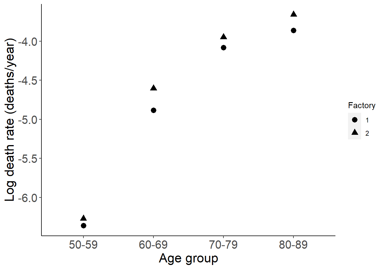

图 38.1: Rates increase with age and age specific rates are higher in factory 2.

都可以看出，死亡率随年龄增长而增加，2号工厂的死亡率似乎在各个年龄组都较1号工厂高。

38.6.3 请用数学语言描述死亡率和年龄组之间关系的模型。

令 \(Y_i\) 为年龄组 \(i, (i = 1,\dots,8)\) 死亡人数，对应的观测时间则为 \(t_i\) 年。如果前提条件每名工人之间相互独立可以认为得到满足，那么 \(Y_i\) 可以用一个死亡率为 \(\lambda_i\) 的泊松模型来描述：

\[ Y_i \sim \text{Po}(\mu_i) \text{ where } \mu_i = \lambda_i t_i \]

对应的链接方程以及其线性预测变量之间的关系可以表述为：

\[ \begin{aligned} \eta_i & = \log(\mu_i) = \log(t_i) + \beta_0 + \beta_1x_{1i} + \beta_2x_{2i} + \beta_3x_{3i} \\ \text{where } x_{1i} & = \left\{ \begin{array}{ll} 0 \text{ if the } i \text{th group is not aged 60-69}\\ 1 \text{ if the } i \text{th group is aged 60-69}\\ \end{array} \right. \\ \text{where } x_{2i} & = \left\{ \begin{array}{ll} 0 \text{ if the } i \text{th group is not aged 70-79}\\ 1 \text{ if the } i \text{th group is aged 70-79}\\ \end{array} \right. \\ \text{where } x_{3i} & = \left\{ \begin{array}{ll} 0 \text{ if the } i \text{th group is not aged 80-89}\\ 1 \text{ if the } i \text{th group is aged 80-89}\\ \end{array} \right. \\ \end{aligned} \]

38.6.3.1 用R和Stata计算上述数学模型描述的死亡率和年龄之间关系的极大似然估计 (MLE)。年龄对于死亡率的效果有多强？

# fit a model without "agegroup"
mA <- glm(n_deaths ~ offset(log(Pyears)), 
              family = poisson(link = "log"), data = Rubber)
jtools::summ(mA, confint = TRUE, digits = 6)

Observations	8
Dependent variable	n_deaths
Type	Generalized linear model
Family	poisson
Link	log

χ²(0)	-0.000000
Pseudo-R² (Cragg-Uhler)	0.000000
Pseudo-R² (McFadden)	0.000000
AIC	142.725329
BIC	142.804771

	Est.	2.5%	97.5%	z val.	p
(Intercept)	-4.795015	-4.949964	-4.640067	-60.652699	0.000000
Standard errors: MLE

# fit a model with age group
mB <- glm(n_deaths ~ Agegrp + offset(log(Pyears)), 
              family = poisson(link = "log"), data = Rubber)
jtools::summ(mB, confint = TRUE, digits = 6)

Observations	8
Dependent variable	n_deaths
Type	Generalized linear model
Family	poisson
Link	log

χ²(3)	102.171839
Pseudo-R² (Cragg-Uhler)	0.999997
Pseudo-R² (McFadden)	0.726037
AIC	46.553491
BIC	46.871257

	Est.	2.5%	97.5%	z val.	p
(Intercept)	-6.315875	-6.839697	-5.792052	-23.631839	0.000000
Agegrp60-69	1.582833	1.004549	2.161118	5.364657	0.000000
Agegrp70-79	2.302963	1.725477	2.880448	7.816170	0.000000
Agegrp80-89	2.554674	1.847314	3.262034	7.078532	0.000000
Standard errors: MLE

lrtest(mA, mB)

Likelihood ratio test

Model 1: n_deaths ~ offset(log(Pyears))
Model 2: n_deaths ~ Agegrp + offset(log(Pyears))
  #Df  LogLik Df  Chisq Pr(>Chisq)    
1   1 -70.363                         
2   4 -19.277  3 102.17  < 2.2e-16 ***
---
Signif. codes:  0 '***' 0.001 '**' 0.01 '*' 0.05 '.' 0.1 ' ' 1

你可以比较加入年龄和没加入年龄时的两个模型，如上面使用的似然比检验法 (likelihood ratio test)。

在 Stata 你可以这样做上面相同的事：

(8 observations read)



Iteration 0:   log likelihood =  -76.82037  
Iteration 1:   log likelihood = -70.363937  
Iteration 2:   log likelihood = -70.362666  
Iteration 3:   log likelihood = -70.362666  

Generalized linear models                          No. of obs      =         8
Optimization     : ML                              Residual df     =         7
                                                   Scale parameter =         1
Deviance         =  103.8826147                    (1/df) Deviance =  14.84037
Pearson          =  103.4540571                    (1/df) Pearson  =  14.77915

Variance function: V(u) = u                        [Poisson]
Link function    : g(u) = ln(u)                    [Log]

                                                   AIC             =  17.84067
Log likelihood   =  -70.3626661                    BIC             =  89.32652

------------------------------------------------------------------------------
             |                 OIM
      deaths |      Coef.   Std. Err.      z    P>|z|     [95% Conf. Interval]
-------------+----------------------------------------------------------------
       _cons |  -4.795015   .0790569   -60.65   0.000    -4.949964   -4.640067
       lpyrs |          1  (offset)
------------------------------------------------------------------------------



Iteration 0:   log likelihood = -19.667375  
Iteration 1:   log likelihood = -19.277924  
Iteration 2:   log likelihood = -19.276748  
Iteration 3:   log likelihood = -19.276748  

Generalized linear models                          No. of obs      =         8
Optimization     : ML                              Residual df     =         4
                                                   Scale parameter =         1
Deviance         =  1.710778974                    (1/df) Deviance =  .4276947
Pearson          =  1.704679988                    (1/df) Pearson  =    .42617

Variance function: V(u) = u                        [Poisson]
Link function    : g(u) = ln(u)                    [Log]

                                                   AIC             =  5.819187
Log likelihood   = -19.27674826                    BIC             = -6.606987

------------------------------------------------------------------------------
             |                 OIM
      deaths |      Coef.   Std. Err.      z    P>|z|     [95% Conf. Interval]
-------------+----------------------------------------------------------------
      agegrp |
          2  |   1.582834   .2950484     5.36   0.000     1.004549    2.161118
          3  |   2.302963   .2946408     7.82   0.000     1.725477    2.880448
          4  |   2.554674   .3609046     7.08   0.000     1.847314    3.262034
             |
       _cons |  -6.315874   .2672612   -23.63   0.000    -6.839697   -5.792052
       lpyrs |          1  (offset)
------------------------------------------------------------------------------



Likelihood-ratio test                                 LR chi2(3)  =    102.17
(Assumption: A nested in B)                           Prob > chi2 =    0.0000

其实Stata里面还可以用简化的 Poisson 命令

(8 observations read)



Iteration 0:   log likelihood = -19.280832  
Iteration 1:   log likelihood = -19.276746  
Iteration 2:   log likelihood = -19.276745  

Poisson regression                                Number of obs   =          8
                                                  LR chi2(3)      =     102.17
                                                  Prob > chi2     =     0.0000
Log likelihood = -19.276745                       Pseudo R2       =     0.7260

------------------------------------------------------------------------------
      deaths |      Coef.   Std. Err.      z    P>|z|     [95% Conf. Interval]
-------------+----------------------------------------------------------------
      agegrp |
          2  |   1.582833   .2950484     5.36   0.000     1.004549    2.161118
          3  |   2.302962   .2946408     7.82   0.000     1.725477    2.880448
          4  |   2.554674   .3609046     7.08   0.000     1.847314    3.262034
             |
       _cons |  -6.315874   .2672612   -23.63   0.000    -6.839697   -5.792052
    ln(pyrs) |          1  (exposure)
------------------------------------------------------------------------------

38.6.3.2 计算下列两组年龄组对比之下的模型估计死亡率比 (rate ratios)

60-69岁比 50-59岁 RR 及其 95%CI

\[ \exp(1.583) (\exp(1.005), \exp(2.161)) = 4.87 (2.73, 8.68) \]

80-89岁比 70-79岁 RR 及其 95%CI 的计算

\[ \exp(\hat{\beta_3} - \hat{\beta_2}) = \exp(2.555 - 2.302) = 1.29 \]

为了获取\(\hat{\beta_3} - \hat{\beta_2}\) 的方差，已知\(\text{Var}(\hat{\beta_3} - \hat{\beta_2}) = \text{Var}( \hat{\beta_3}) + \text{Var}(\hat{\beta_2}) - 2\text{Cov}(\hat{\beta_3}, \hat{\beta_2})\)。根据这个在概率论学到的方差性质，我们可以手动计算想要的方差和标准差，从而进一步获取其 95% CI：

You can also use vce command in Stata to obtain the Covariance matrix of coefficients of a fitted poisson model

vcov(mB)

            (Intercept) Agegrp60-69 Agegrp70-79 Agegrp80-89
(Intercept)  0.07142857 -0.07142857 -0.07142857 -0.07142857
Agegrp60-69 -0.07142857  0.08705357  0.07142857  0.07142857
Agegrp70-79 -0.07142857  0.07142857  0.08681319  0.07142857
Agegrp80-89 -0.07142857  0.07142857  0.07142857  0.13025210

\[ \begin{aligned} \text{Var}(\hat{\beta_3} - \hat{\beta_2}) & = \text{Var}(\hat{\beta_3}) + \text{Var}(\hat{\beta_2}) - 2\text{Cov}(\hat{\beta_3}, \hat{\beta_2}) \\ & = 0.13025 + 0.08681 - 2 \times 0.07143 \\ & = 0.0743 \\ \Rightarrow \text{the 95%CI} & = \exp(2.555 - 2.303 \pm\sqrt{0.07143}) \\ & = (0.75, 2.20) \end{aligned} \]

在R里你可以这样计算：

# change the reference group to "70-79"
Rubber <- Rubber %>% 
  mutate(Agegrp1 = fct_relevel(Agegrp, "70-79"))

mC <- glm(n_deaths ~ Agegrp1 + offset(log(Pyears)), 
              family = poisson(link = "log"), data = Rubber)
jtools::summ(mC, confint = TRUE, digits = 6, exp = TRUE)

Observations	8
Dependent variable	n_deaths
Type	Generalized linear model
Family	poisson
Link	log

χ²(3)	102.171839
Pseudo-R² (Cragg-Uhler)	0.999997
Pseudo-R² (McFadden)	0.726037
AIC	46.553491
BIC	46.871257

	exp(Est.)	2.5%	97.5%	z val.	p
(Intercept)	0.018081	0.014179	0.023056	-32.353131	0.000000
Agegrp150-59	0.099962	0.056110	0.178088	-7.816170	0.000000
Agegrp160-69	0.486689	0.344635	0.687297	-4.089424	0.000043
Agegrp180-89	1.286225	0.754119	2.193786	0.924013	0.355480
Standard errors: MLE

但是在 Stata 里面可以使用灵活无比的 lincom 命令：

(8 observations read)




 ( 1)  - [deaths]3.agegrp + [deaths]4.agegrp = 0

------------------------------------------------------------------------------
      deaths |     exp(b)   Std. Err.      z    P>|z|     [95% Conf. Interval]
-------------+----------------------------------------------------------------
         (1) |   1.286225   .3503829     0.92   0.355     .7541189    2.193786
------------------------------------------------------------------------------

38.6.4 接下来的模型中在前面的基础上加入工厂编号，你认为是否有证据证明工厂之间的工人的死亡率在调整了年龄之后依然有差异？计算年龄调整过后的两工厂之间死亡率之比和95%CI。

mD <- glm(n_deaths ~ Agegrp + Factory + offset(log(Pyears)), 
              family = poisson(link = "log"), data = Rubber)
jtools::summ(mD, confint = TRUE, digits = 6, exp = TRUE)

Observations	8
Dependent variable	n_deaths
Type	Generalized linear model
Family	poisson
Link	log

χ²(4)	103.666936
Pseudo-R² (Cragg-Uhler)	0.999998
Pseudo-R² (McFadden)	0.736662
AIC	47.058393
BIC	47.455601

	exp(Est.)	2.5%	97.5%	z val.	p
(Intercept)	0.001640	0.000947	0.002839	-22.900655	0.000000
Agegrp60-69	4.839413	2.714014	8.629254	5.343443	0.000000
Agegrp70-79	9.949876	5.584586	17.727369	7.796966	0.000000
Agegrp80-89	12.864610	6.341532	26.097509	7.077995	0.000000
Factory2	1.213953	0.888998	1.657687	1.219745	0.222561
Standard errors: MLE

lrtest(mD, mB)

Likelihood ratio test

Model 1: n_deaths ~ Agegrp + Factory + offset(log(Pyears))
Model 2: n_deaths ~ Agegrp + offset(log(Pyears))
  #Df  LogLik Df  Chisq Pr(>Chisq)
1   5 -18.529                     
2   4 -19.277 -1 1.4951     0.2214

从 mD 模型的报告来看，2号工厂比较1号工厂的工人死亡率比是 1.21 (95%CI: 0.89, 1.66)。两个模型的似然比检验结果也提示，并无确实证据证明两工厂工人的死亡率在调整了年龄因素之后有显著差异。

38.6.5 现在在前一步加了工厂变量的基础上，重新拟合模型，加入工厂和年龄之间的交互作用项

mE <- glm(n_deaths ~ Agegrp + Factory + Factory*Agegrp 
                    + offset(log(Pyears)), 
              family = poisson(link = "log"), data = Rubber)
summary(mE); jtools::summ(mE, confint = TRUE, digits = 6, exp = TRUE)


Call:
glm(formula = n_deaths ~ Agegrp + Factory + Factory * Agegrp + 
    offset(log(Pyears)), family = poisson(link = "log"), data = Rubber)

Coefficients:
                     Estimate Std. Error z value Pr(>|z|)    
(Intercept)          -6.35933    0.37796 -16.825  < 2e-16 ***
Agegrp60-69           1.47456    0.42414   3.477 0.000508 ***
Agegrp70-79           2.27784    0.41975   5.427 5.74e-08 ***
Agegrp80-89           2.49597    0.51755   4.823 1.42e-06 ***
Factory2              0.08888    0.53452   0.166 0.867939    
Agegrp60-69:Factory2  0.19018    0.59142   0.322 0.747789    
Agegrp70-79:Factory2  0.04246    0.58959   0.072 0.942587    
Agegrp80-89:Factory2  0.11377    0.72237   0.157 0.874854    
---
Signif. codes:  0 '***' 0.001 '**' 0.01 '*' 0.05 '.' 0.1 ' ' 1

(Dispersion parameter for poisson family taken to be 1)

    Null deviance: 1.0388e+02  on 7  degrees of freedom
Residual deviance: 1.1990e-14  on 0  degrees of freedom
AIC: 52.843

Number of Fisher Scoring iterations: 3

Observations	8
Dependent variable	n_deaths
Type	Generalized linear model
Family	poisson
Link	log

χ²(7)	103.882612
Pseudo-R² (Cragg-Uhler)	0.999998
Pseudo-R² (McFadden)	0.738194
AIC	52.842718
BIC	53.478250

	exp(Est.)	2.5%	97.5%	z val.	p
(Intercept)	0.001731	0.000825	0.003630	-16.825197	0.000000
Agegrp60-69	4.369124	1.902683	10.032807	3.476599	0.000508
Agegrp70-79	9.755607	4.285111	22.209899	5.426658	0.000000
Agegrp80-89	12.133483	4.399941	33.459862	4.822670	0.000001
Factory2	1.092948	0.383366	3.115916	0.166276	0.867939
Agegrp60-69:Factory2	1.209461	0.379467	3.854873	0.321556	0.747789
Agegrp70-79:Factory2	1.043376	0.328533	3.313620	0.072019	0.942587
Agegrp80-89:Factory2	1.120495	0.271972	4.616327	0.157495	0.874854
Standard errors: MLE

38.6.5.1 请问这是一个怎样的模型？

这是一个有8组观测数据，8个参数估计的模型，是一个饱和模型。 The model is saturated.

38.6.5.2 有没有足够的证据证明工厂和年龄变量之间的交互作用项是有意义的？

lrtest(mE, mD)

Likelihood ratio test

Model 1: n_deaths ~ Agegrp + Factory + Factory * Agegrp + offset(log(Pyears))
Model 2: n_deaths ~ Agegrp + Factory + offset(log(Pyears))
  #Df  LogLik Df  Chisq Pr(>Chisq)
1   8 -18.421                     
2   5 -18.529 -3 0.2157      0.975

似然比检验结果显示，没有证据证明二者之间交互作用项是有意义的。

38.6.5.3 用数学语言描述上述包含了交互作用项的模型，并利用这个模型手头计算下列各组的死亡率：

1号工厂的 70-79 岁
2号工厂的 50-50 岁
2号工厂的 60-69 岁

\[ \begin{aligned} \eta_i = \log(\mu_i) & = \log(t_i) + \beta_0 + \beta_1x_{1i} + \beta_2x_{2i} + \beta_3x_{3i} + \beta_4z_{i} \\ & \;\;\; + \beta_5(x_{1i}z_{i}) + \beta_6(x_{2i}z_{i}) + \beta_7(x_{3i}z_{i})\\ \text{where } x_{1i} & = \left\{ \begin{array}{ll} 0 \text{ if the } i \text{th group is not aged 60-69}\\ 1 \text{ if the } i \text{th group is aged 60-69}\\ \end{array} \right. \\ \text{where } x_{2i} & = \left\{ \begin{array}{ll} 0 \text{ if the } i \text{th group is not aged 70-79}\\ 1 \text{ if the } i \text{th group is aged 70-79}\\ \end{array} \right. \\ \text{where } x_{3i} & = \left\{ \begin{array}{ll} 0 \text{ if the } i \text{th group is not aged 80-89}\\ 1 \text{ if the } i \text{th group is aged 80-89}\\ \end{array} \right. \\ \text{and } z_{i} & = \left\{ \begin{array}{ll} 0 \text{ if the } i \text{th group is from factory 1}\\ 1 \text{ if the } i \text{th group is from factory 2}\\ \end{array} \right. \end{aligned} \]

1号工厂的 70-79 岁组中该模型估计的死亡率是

\[ \exp(\hat{\beta}_0 + \hat{\beta}_2) = \exp(-6.359 + 2.2778) = 16.9 /1000 \text{ person-years} \]

2号工厂的 50-59 岁组中该模型估计的死亡率是

\[ \exp(\hat{\beta}_0 + \hat{\beta}_4) = \exp(-6.359 + 0.089) = 1.89 / 1000 \text{ person-years} \]

2号工厂的 60-69 岁组中该模型估计的死亡率是

\[ \exp(\hat{\beta}_0 + \hat{\beta}_1 + \hat{\beta}_4 + \hat{\beta}_5) = \exp(-6.359 + 1.475 + 0.089 + 0.190) = 10.0 / 1000 \text{ person-years} \]

38.6.5.4 对比你计算的模型估计死亡率和实际观测到的死亡率

tab <- Epi::stat.table(index=list(Factory=Factory,Agegrp=Agegrp),
                   contents=list(sum(n_deaths/Pyears)), 
                  data=Rubber, margins=FALSE)

print(tab, digits = 7)

 -------------------------------------------------- 
          -----------------Agegrp------------------ 
 Factory       50-59     60-69     70-79     80-89  
 -------------------------------------------------- 
 1         0.0017305 0.0075609 0.0168824 0.0209974  
 2         0.0018914 0.0099946 0.0192519 0.0257143  
 --------------------------------------------------

我们发现该模型估计的各组的死亡率和观测值完全一致。

38.6.6 现在把年龄当作连续型变量来考虑。拟合下列模型

38.6.6.1 只有年龄作为连续型变量

mF <- glm(n_deaths ~ as.numeric(Agegrp) + offset(log(Pyears)), 
              family = poisson(link = "log"), data = Rubber)
jtools::summ(mF, confint = TRUE, digits = 6, exp = TRUE)

Observations	8
Dependent variable	n_deaths
Type	Generalized linear model
Family	poisson
Link	log

χ²(1)	89.442531
Pseudo-R² (Cragg-Uhler)	0.999986
Pseudo-R² (McFadden)	0.635582
AIC	55.282799
BIC	55.441682

	exp(Est.)	2.5%	97.5%	z val.	p
(Intercept)	0.001421	0.000910	0.002217	-28.874573	0.000000
as.numeric(Agegrp)	2.239658	1.899333	2.640963	9.588396	0.000000
Standard errors: MLE

mF 的结果提供很强的证据证明年龄作为连续型变量和死亡率的变化有关。年龄每增加10岁，死亡率增长的数字要乘以 2.24。

38.6.6.2 年龄和工厂两个预测变量

mG <- glm(n_deaths ~ as.numeric(Agegrp) + Factory + offset(log(Pyears)), 
              family = poisson(link = "log"), data = Rubber)
jtools::summ(mG, confint = TRUE, digits = 6, exp = TRUE)

Observations	8
Dependent variable	n_deaths
Type	Generalized linear model
Family	poisson
Link	log

χ²(2)	91.170538
Pseudo-R² (Cragg-Uhler)	0.999989
Pseudo-R² (McFadden)	0.647862
AIC	55.554792
BIC	55.793116

	exp(Est.)	2.5%	97.5%	z val.	p
(Intercept)	0.001274	0.000790	0.002053	-27.358186	0.000000
as.numeric(Agegrp)	2.239890	1.899067	2.641880	9.575477	0.000000
Factory2	1.231652	0.902034	1.681716	1.311155	0.189805
Standard errors: MLE

lrtest(mG, mF)

Likelihood ratio test

Model 1: n_deaths ~ as.numeric(Agegrp) + Factory + offset(log(Pyears))
Model 2: n_deaths ~ as.numeric(Agegrp) + offset(log(Pyears))
  #Df  LogLik Df Chisq Pr(>Chisq)
1   3 -24.777                    
2   2 -25.641 -1 1.728     0.1887

并无有效证据证明工厂之间有死亡率的显著区别。

38.6.6.3 年龄和工厂，及两个变量的交互作用项

mH <- glm(n_deaths ~ as.numeric(Agegrp) + Factory  + as.numeric(Agegrp)*Factory + 
          offset(log(Pyears)), family = poisson(link = "log"), data = Rubber)
jtools::summ(mH, confint = TRUE, digits = 6, exp = TRUE)

Observations	8
Dependent variable	n_deaths
Type	Generalized linear model
Family	poisson
Link	log

χ²(3)	91.183730
Pseudo-R² (Cragg-Uhler)	0.999989
Pseudo-R² (McFadden)	0.647955
AIC	57.541599
BIC	57.859365

	exp(Est.)	2.5%	97.5%	z val.	p
(Intercept)	0.001240	0.000642	0.002395	-19.936299	0.000000
as.numeric(Agegrp)	2.263303	1.776141	2.884084	6.605055	0.000000
Factory2	1.293657	0.528919	3.164090	0.564224	0.572602
as.numeric(Agegrp):Factory2	0.980790	0.704402	1.365623	-0.114855	0.908560
Standard errors: MLE

lrtest(mG, mH)

Likelihood ratio test

Model 1: n_deaths ~ as.numeric(Agegrp) + Factory + offset(log(Pyears))
Model 2: n_deaths ~ as.numeric(Agegrp) + Factory + as.numeric(Agegrp) * 
    Factory + offset(log(Pyears))
  #Df  LogLik Df  Chisq Pr(>Chisq)
1   3 -24.777                     
2   4 -24.771  1 0.0132     0.9086

并无有效证据证明工厂之间的相互作用项有意义。

38.6.7 计算只有年龄(连续型)和工厂两个变量模型时的模型偏差 (deviance)，该模型和第一部分中饱和模型之间相比相差几个参数(parameters)？你有怎样的推论？

lrtest(mF, mE)

Likelihood ratio test

Model 1: n_deaths ~ as.numeric(Agegrp) + offset(log(Pyears))
Model 2: n_deaths ~ Agegrp + Factory + Factory * Agegrp + offset(log(Pyears))
  #Df  LogLik Df Chisq Pr(>Chisq)  
1   2 -25.641                      
2   8 -18.421  6 14.44    0.02509 *
---
Signif. codes:  0 '***' 0.001 '**' 0.01 '*' 0.05 '.' 0.1 ' ' 1

看上面似然比检验结果显示，有一些不太强的证据 (p = 0.0262) 证明相对饱和模型来说，把年龄当连续变量的模型可能拟合度较差。所以把年龄当作分类型变量 (categorical) 会是比较好的选择。

38.6.8 对这个数据进行了这一系列的分析之后，你从流行病学的角度来说，有怎样的结论？

总的来说，死亡率随着年龄增长而增加。 60-69 岁组的死亡率是50-59 岁组的 4.8 (95% CI 2.7, 8.6) 倍。之后年龄每增长十岁死亡率也在增长，只是增长幅度逐渐减少。至于工厂之间的死亡率比较，2号工厂似乎有 21% 较高 (95%CI: -11%, 66%) 的死亡率。但是工厂之间的死亡率差异并无显著性 (p = 0.22)。交互作用项的分析也表明，并没有证据表明工厂之间的死亡率差异会由于年龄的变化而有所不同。

第 38 章 率的广义线性回归